CS180 Project 2
Introduction
In this project, we are required to experiment with filters and frequency components on various types of images.
Part 1: Filters
1.1: Implementation of convolution
As is known, convolution can be formulated as:
\[
G = H * F, G[i, j]= \sum_{u=-k}^k \sum_{v=-k}^k H[u, v]F[i - u, i - v],
\]
where \(H\) is the kernel, \(F\) is the input image, and \(G\) is the output image.
These are my implementations of convolution, using 4 (conv_1) and 2 (conv_2)
for-loops, respectively:
  import numpy as np

  def conv_1(kernel, img):
    def conv_1(kernel, img):
    h,w = kernel.shape
    k_h = h // 2
    k_w = w // 2
    H, W = img.shape
    img_padded = np.zeros((H + 2 * k_h, W + 2 * k_w))
    img_padded[k_h:-k_h, k_w:-k_w]=img
    img_new = np.zeros_like(img)
    for i in range(H):
        for j in range(W):
            for u in range(-k_h, k_h + 1):
                for v in range(-k_w, k_w + 1):
                    img_new[i, j] += img_padded[i + k_h - u, j + k_w - v] * kernel[u, v]
    return img_new
  import numpy as np

  def conv_2(kernel, img):
    h,w = kernel.shape
    k_h = h // 2
    k_w = w // 2
    H, W = img.shape
    img_padded = np.zeros((H + 2 * k_h, W + 2 * k_w))
    img_padded[k_h:-k_h, k_w:-k_w] = img
    img_new = np.zeros_like(img)
    for i in range(k_h * 2 + 1):
        for j in range(k_w * 2 + 1):
            img_new += img_padded[2 * k_h - i: -i or None, 2 * k_h - j :-j or None] * kernel[i, j]
    return img_new
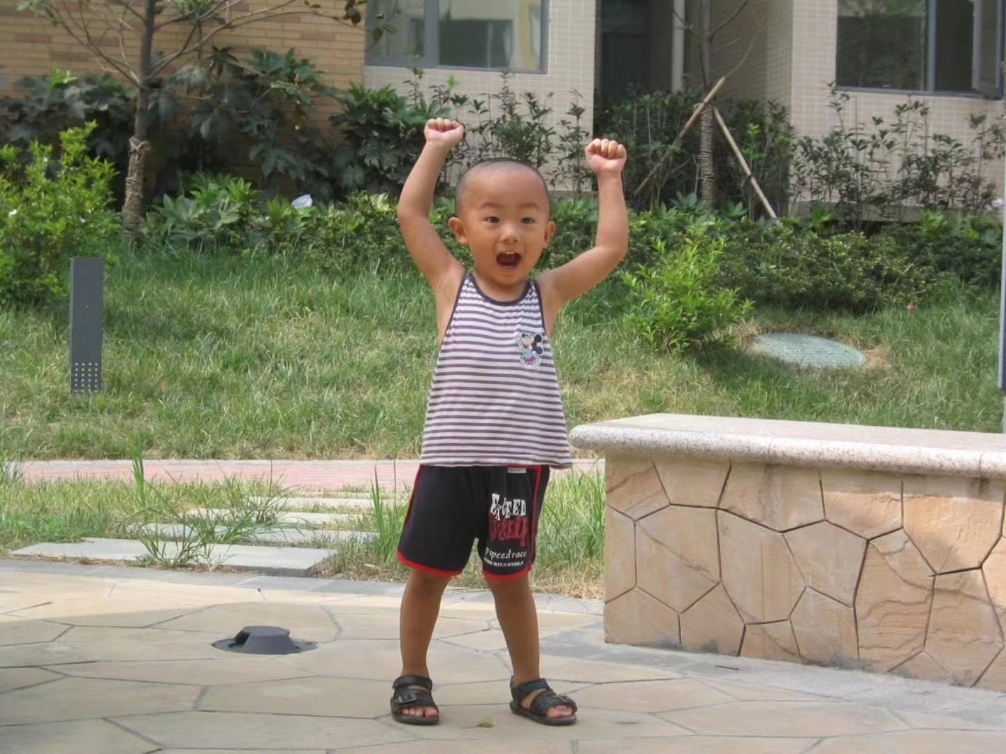
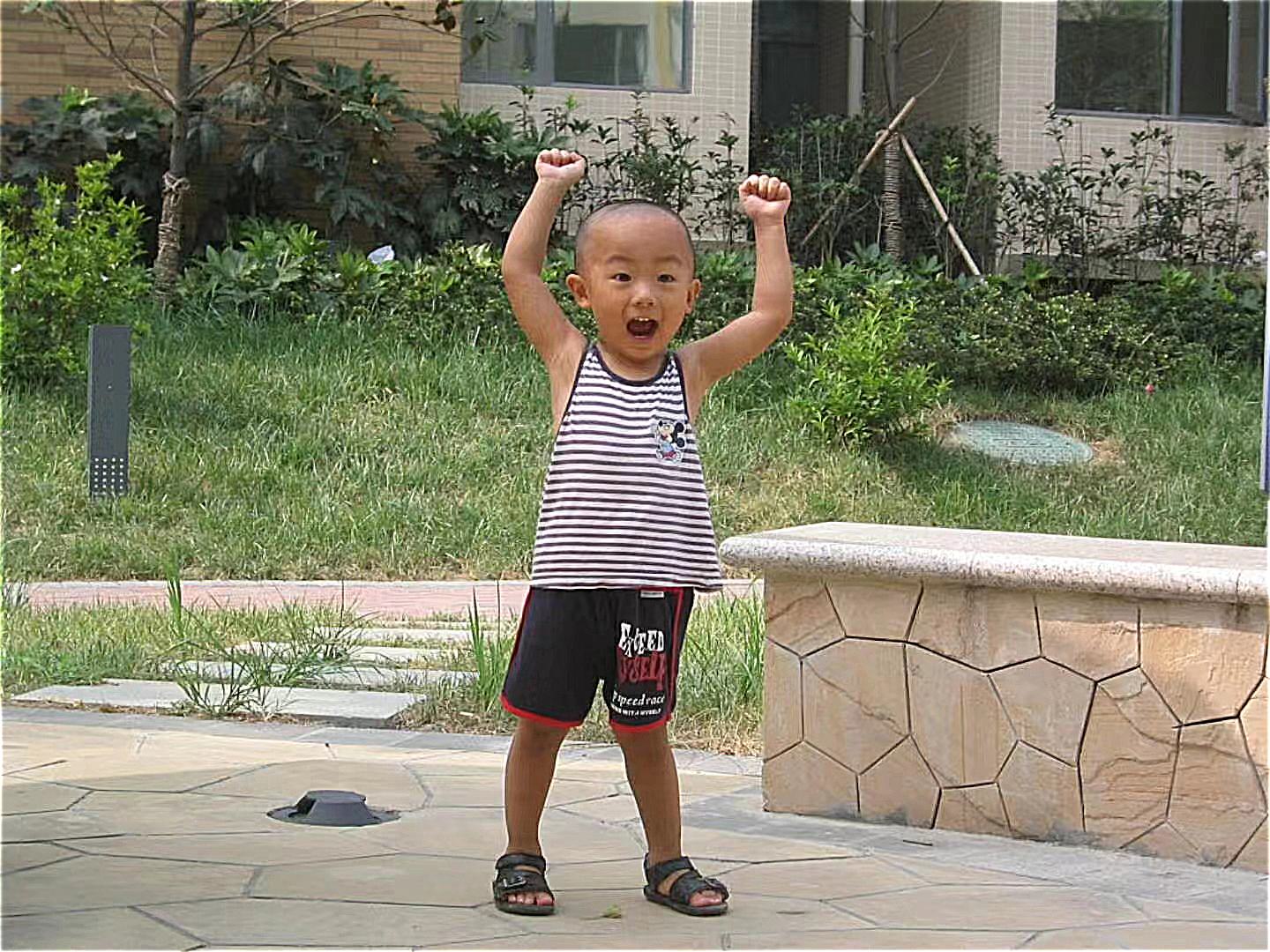
I convolved a picture of myself with the \(9 \times 9\) box filter, using the functions above:


conv_1 runtime: 49.84s
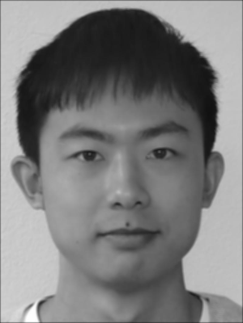
conv_2 runtime: 0.33s
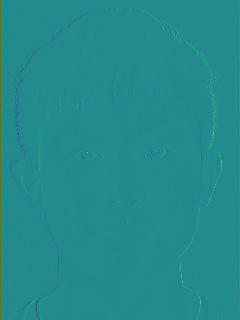
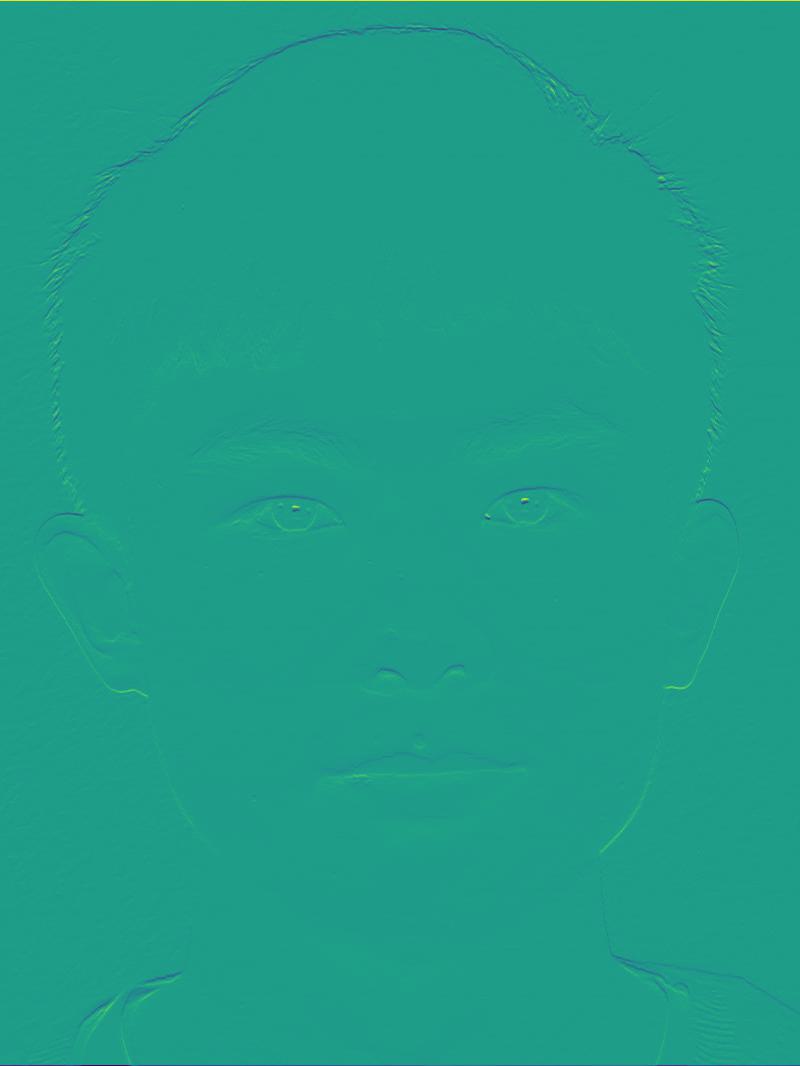
It is clear that conv_2 saves a large amount of time, and here are also convolution results with difference operators \(D_x\) and \(D_y\):
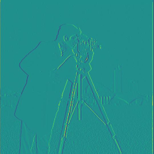
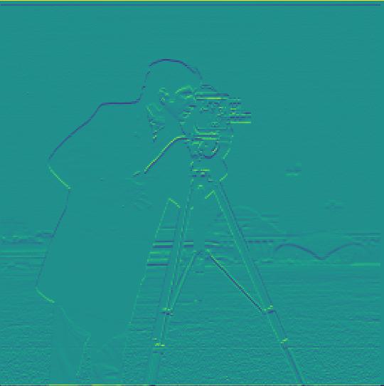
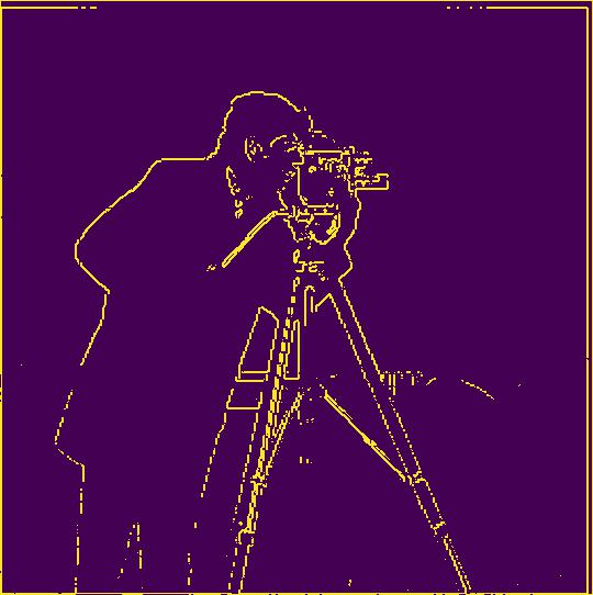
1.2: Finite difference operator
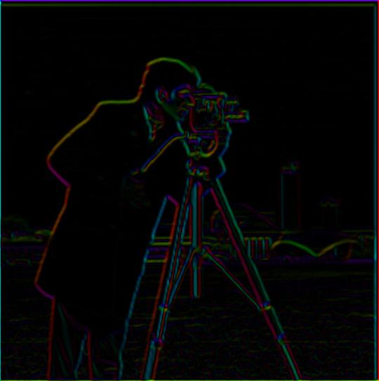
In this section, I primarily experimented with cameraman.jpg, on gradient computation and edge detection
(any pixel with a gradient magnitude larger than a threshold can be considered as on the edge, here by trial, I set it to 0.35):
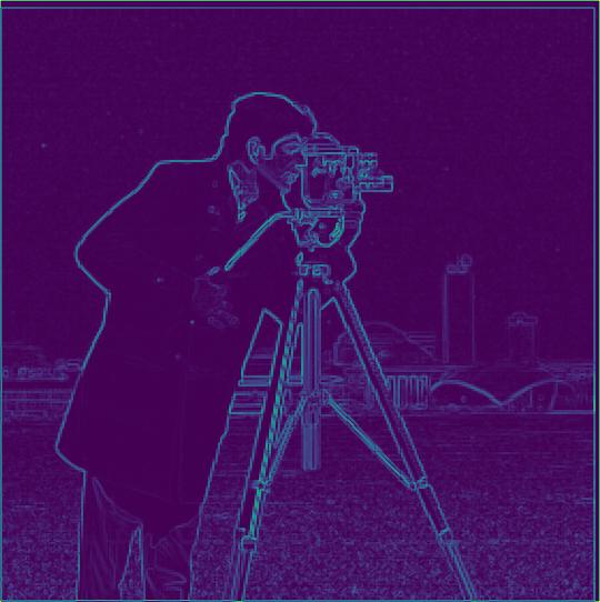
1.3: Derivative of Gaussian (DoG) filter
For smoothing, I use a \(9 \times 9\) Gaussian kernel with \(\sigma = 2\), then I did the gradient computation. We can clearly observe a reduction in noise in the new gradient map. Also, I computed with the DoG filter, with nearly identical outcomes, with a slight difference in the overall magnitudes:
then computed gradient
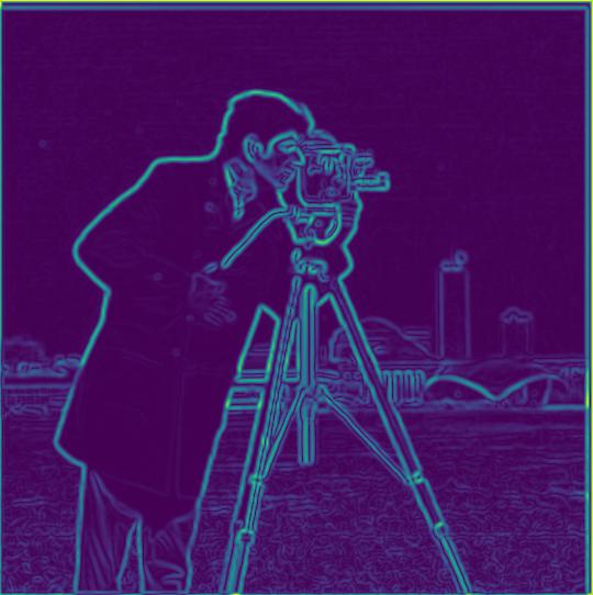
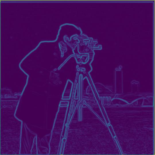
Besides, I visualized the orientations of the pixel gradients with the HSV colorspace, by setting the hue as the gradient vector's angle, saturation as 1, and value as the normalized gradient magnitude:
Part 2: Frequencies
2.1: Image sharpening
In this section, I chose some images to implement sharpening. The sharpening operation can be formulated as: \[ f + \alpha(f - f * g) = f * ((1+\alpha)e - \alpha g), \] where \(f\) is the image, \(g\) is the Gaussian kernel. Here are my sharpening results:
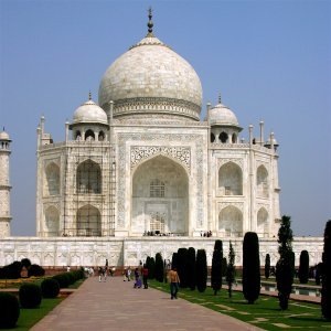
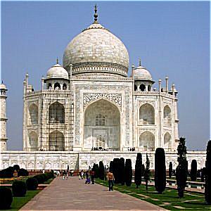
(kernel \(5 \times 5\), \(\sigma = 1.5\), \(\alpha = 1.5\))
(kernel \(9 \times 9\), \(\sigma = 2\), \(\alpha = 2\))
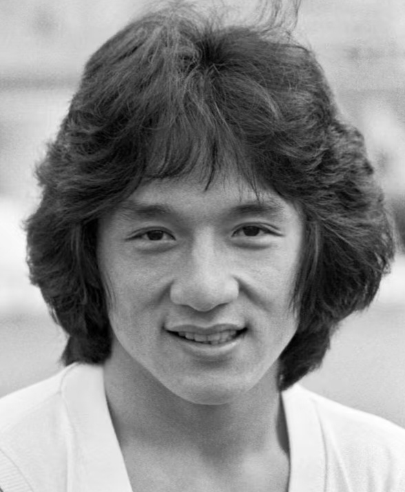
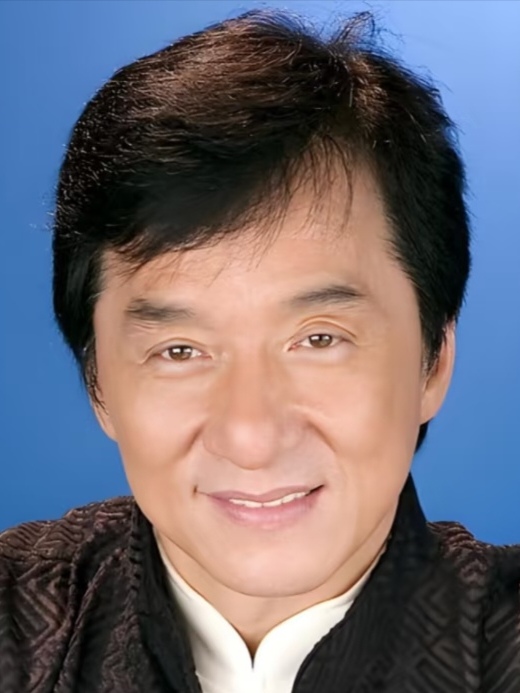
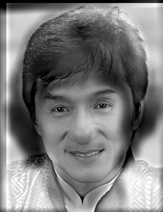
2.2: Hybrid images
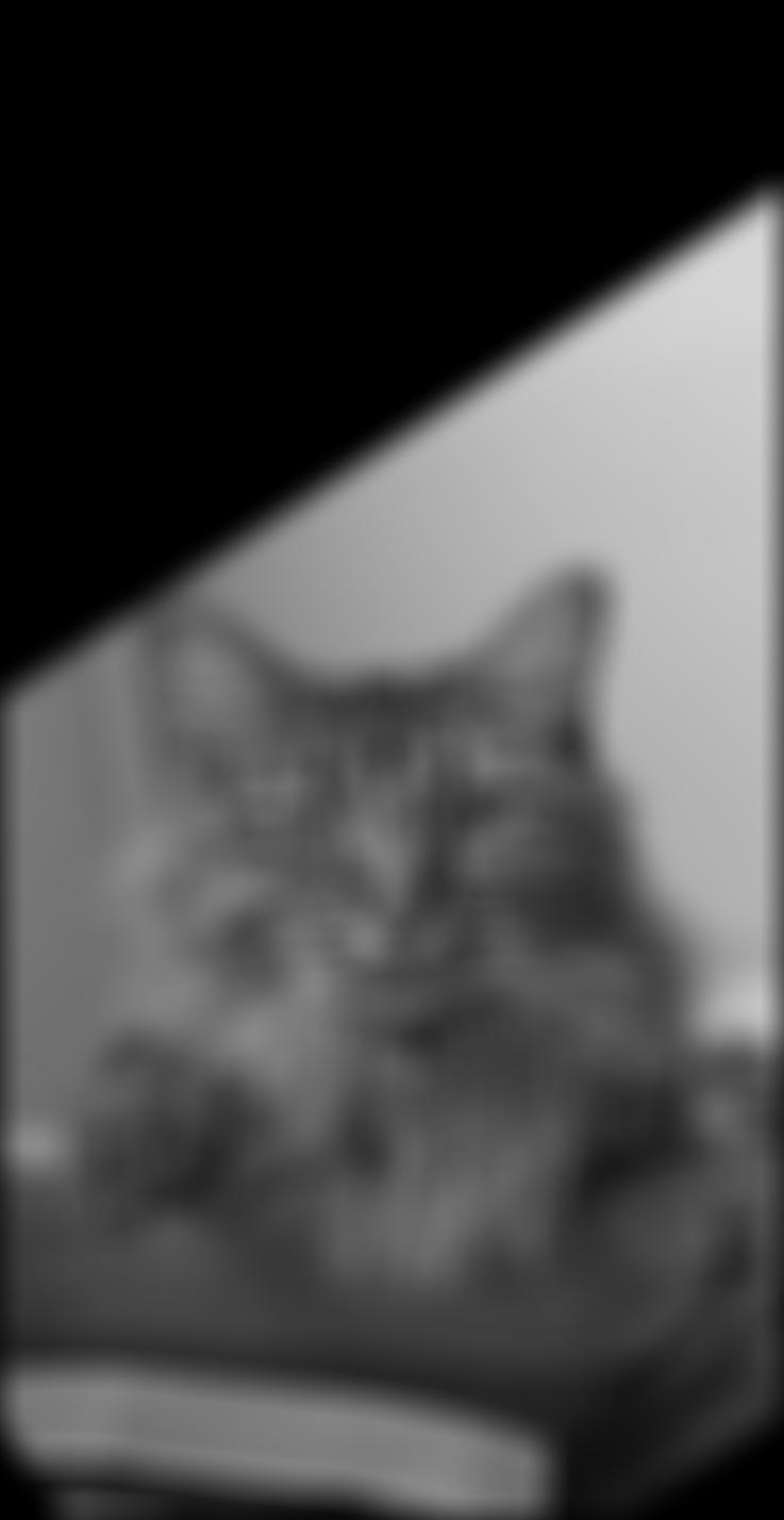
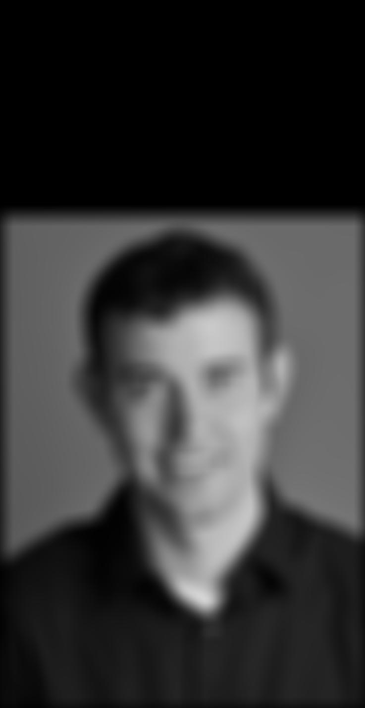
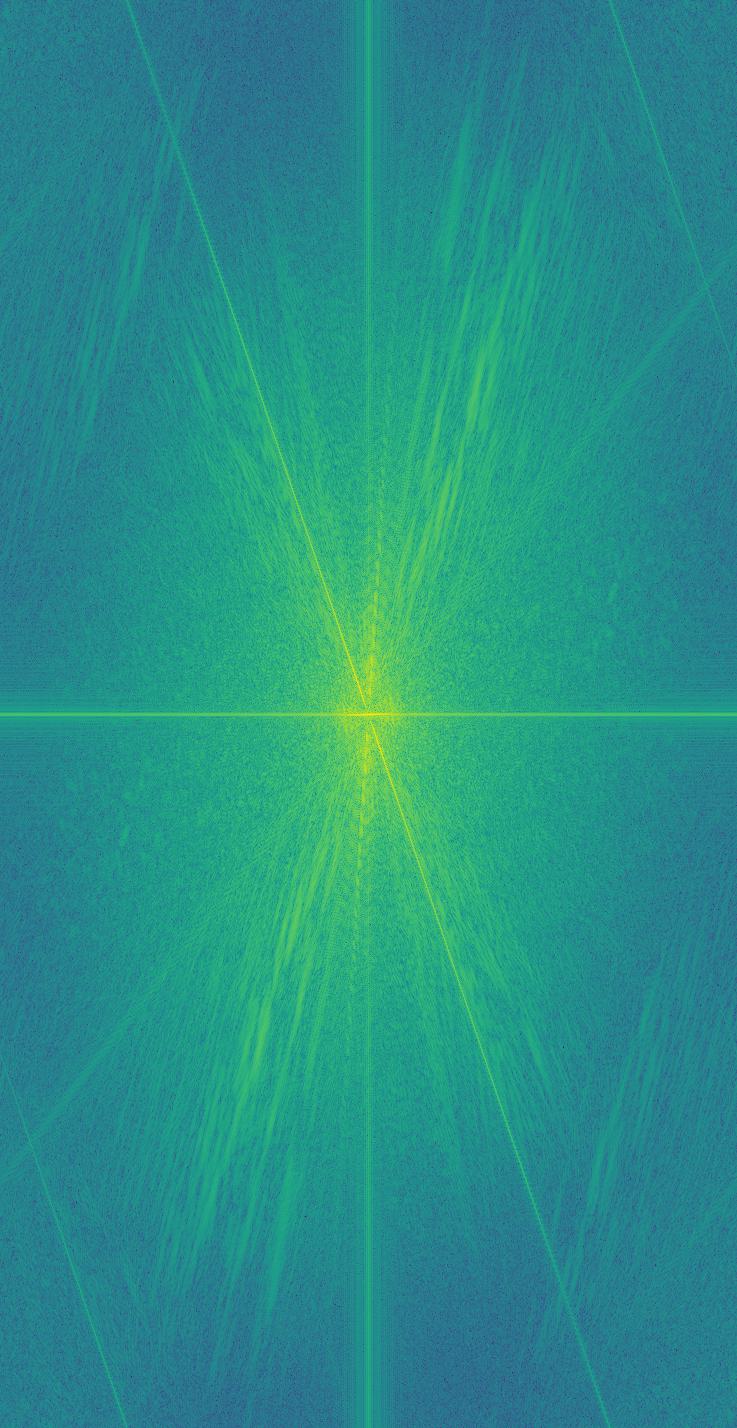
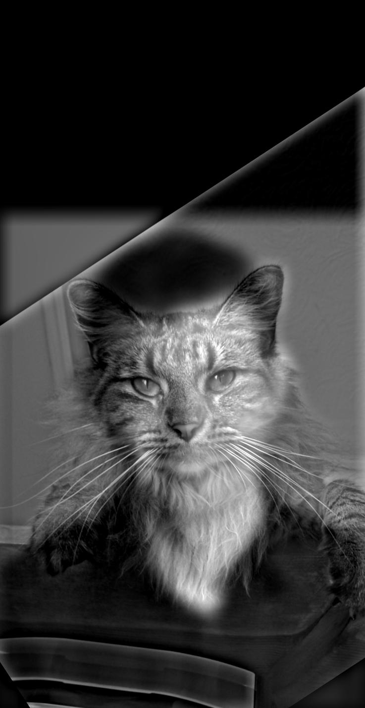
To create a hybrid image, we should blend the high-frequency component of one image with the low-frequency one of the other. Here is the whole procedure of implementation on a pair of example images:
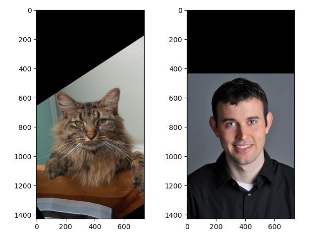
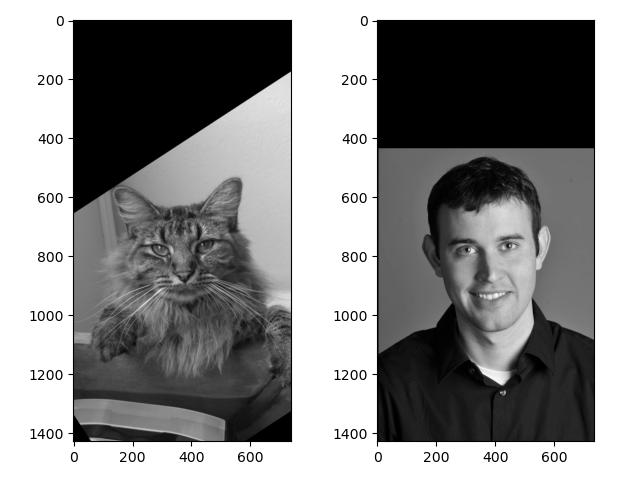
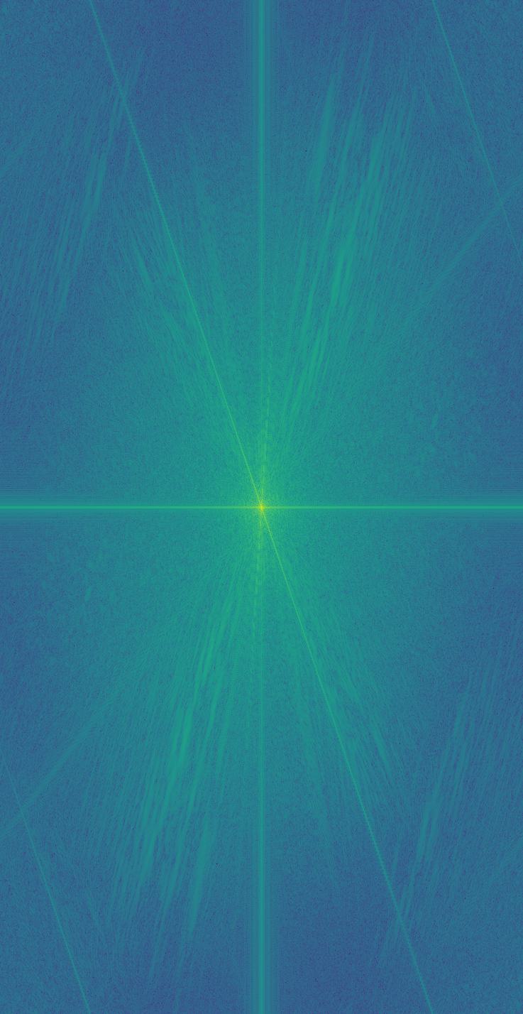
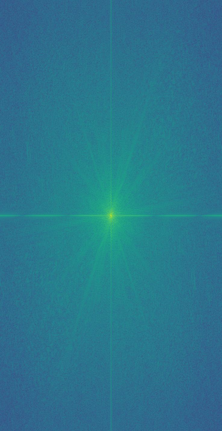
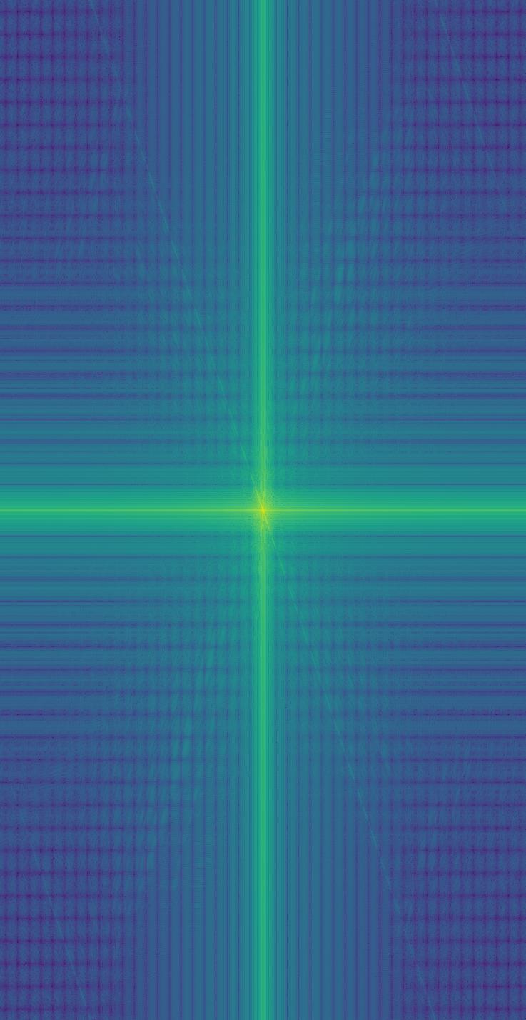
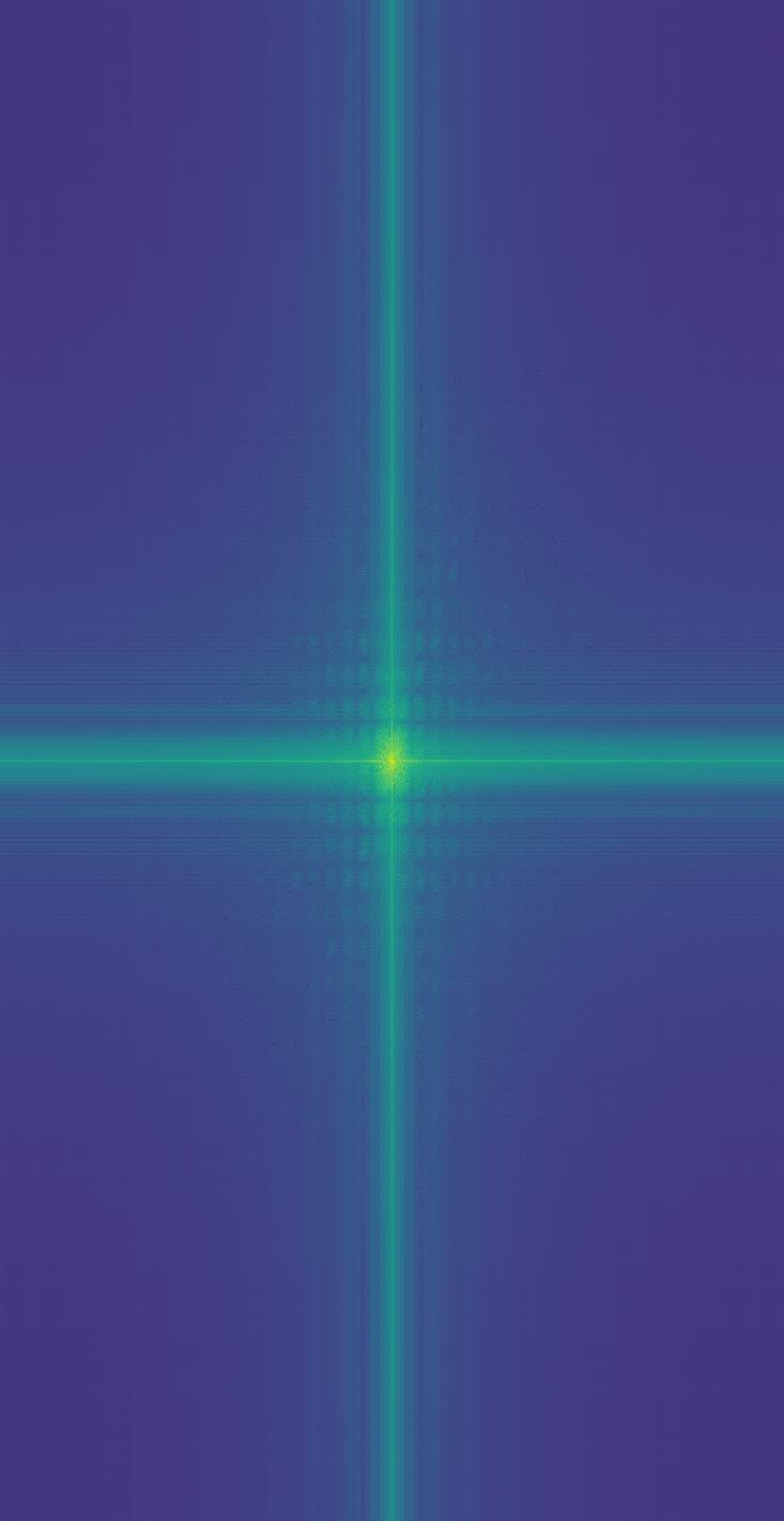
Thus, most high-frequency components are filtered out, and the remaining vertical/horizontal lines in the frequency maps indicate the cropped edges of the images.
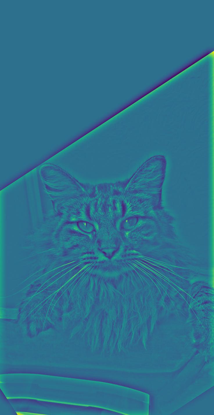
Now, we have our final outcome. When viewed at a short distance, you will see a cat; while standing farther from the image, you will see a blurred man.
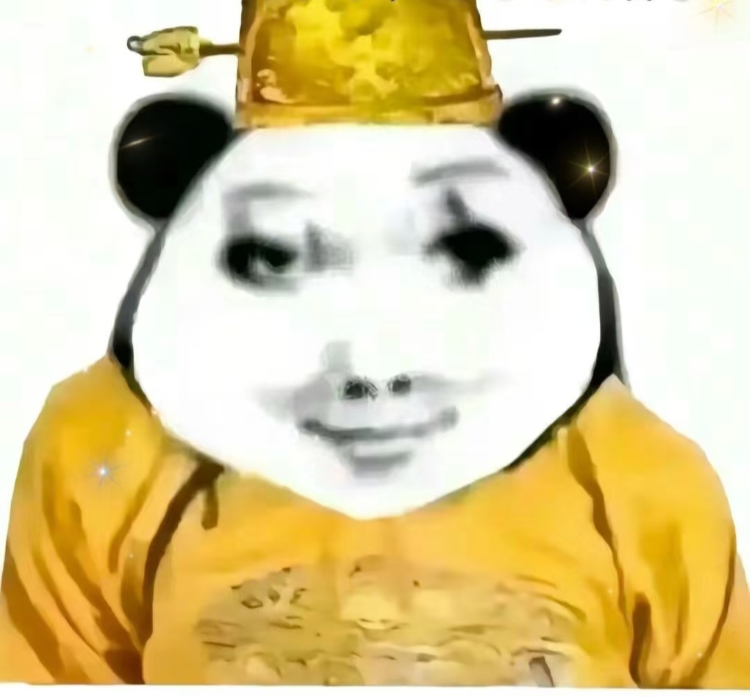
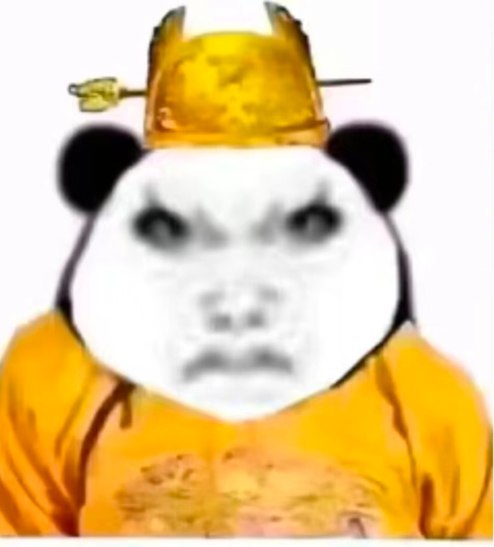
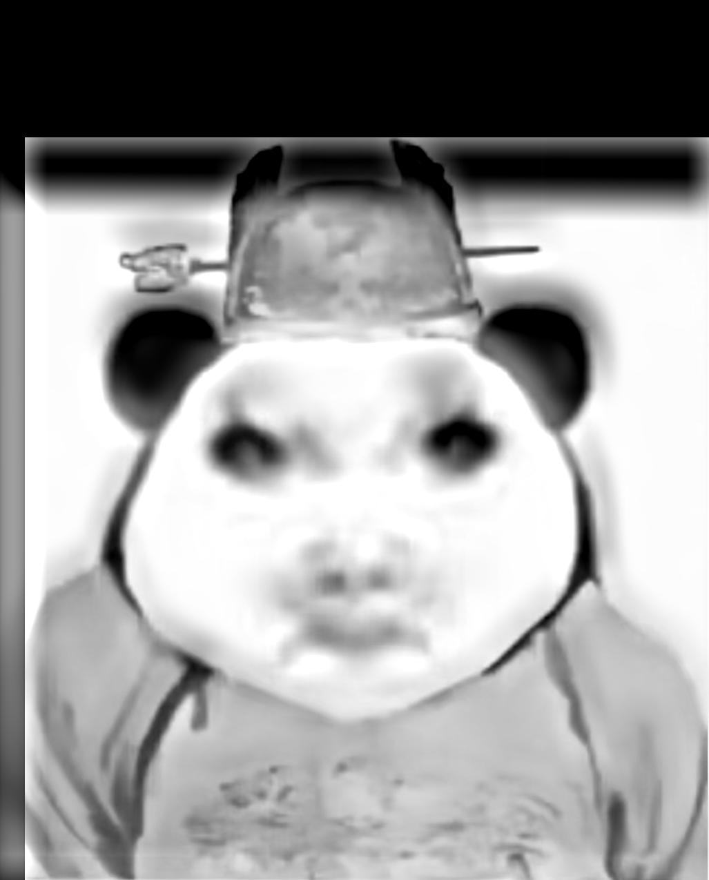
Similarly, we can apply it to other image pairs:
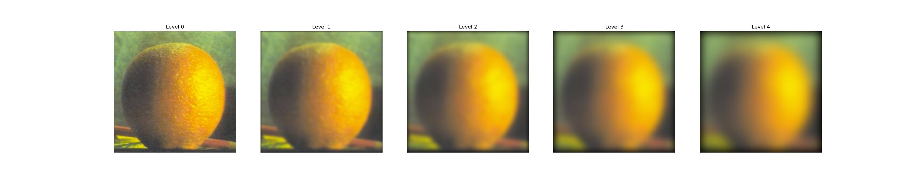
2.3: Gaussian and Laplacian stacks
To build a Gaussian stack, we should filter an image with a Gaussian filter at each level, deriving a sequence of images with increasing extent of blur. Note that the Gaussian filter at higher levels should have larger variance. Here, with the preset base kernel size \(k\) and standard deviation \(\sigma_0\) , at level \(i\) the Gaussian kernel has a size of \(2ik + 1 \times 2ik + 1\) and the \(\sigma_i\) of \(0.5i\sigma_0\).
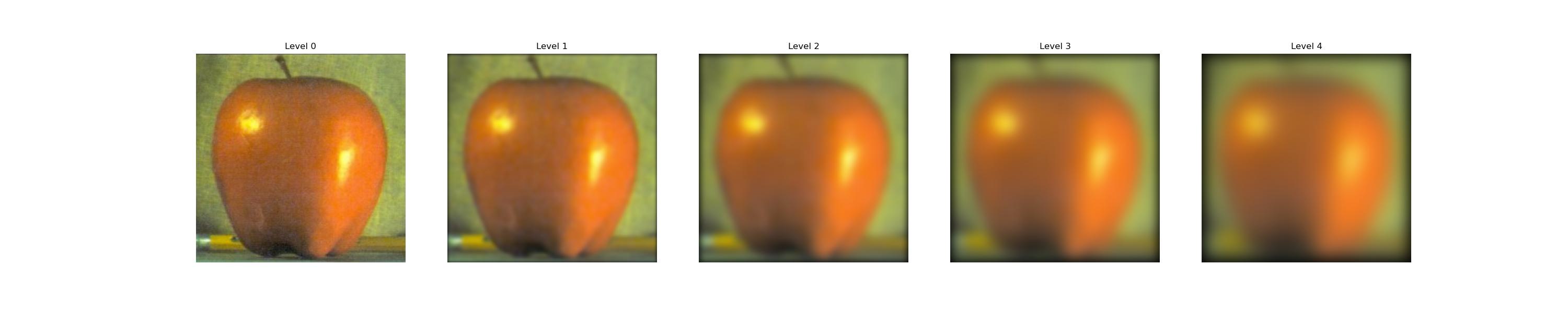
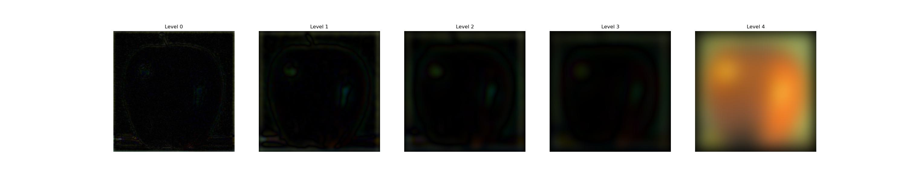
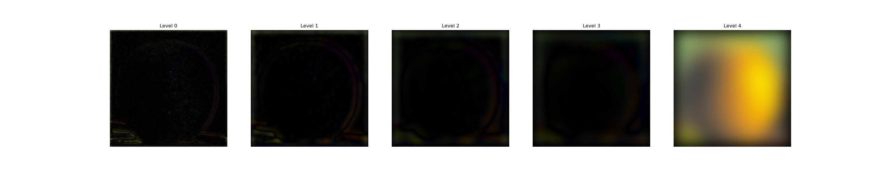
To derive the Laplacian stack, we should leave the most blurred image out as the part with the lowest frequency, and subtract each image from that of a lower level:
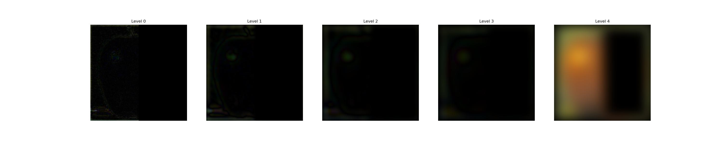
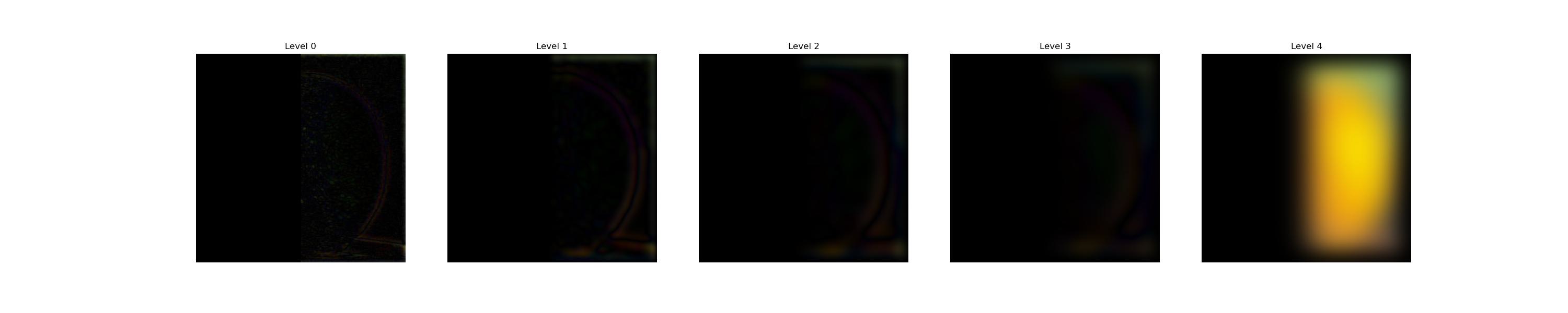
2.4: Multiresolution blending
Now, with the Laplacian stack, as well as a mask \(m\) creating a vertical seam, we can create a Gaussian stack \(G\) of the mask, then multiply each level of it with the corresponding level of image stack \(L_A, L_B\): \[ I_i = m_i \odot I_{A_i} + (1- m_i) \odot I_{B_i}. \]
Thus, with the masks becoming blurrier at higher levels of the stack, there is more overlap between the lower-frequency components of the apple and orange, creating a smoother yet not overly ghosted transition.
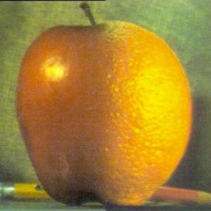
By \(\sum_i I_i\), we will have the final blended image:
Similarly, we can also apply such a technique to scenarios where the masks are in irregular shapes:

Summary
In a word, this project requires patience, especially when implementing those algorithms on my own chosen images, because you have to consider the frequency characteristics of the image in order to have a satisfactory visual effect, and the combination should be interesting as well. Also, finding the edges and generating the irregular masks are not easy. Anyway, it is a really novel experience, because creativity and imagination are combined with the seemingly 'cold'/'plain' coding part.