CS180 Project 3

Part A: Image Warping and Mosaicing

In this part of the project, we are required to conduct the full pipeline of image warping and mosaicing, from deriving transformation matrices to generating new images by sampling.

A.1: Shoot the pictures

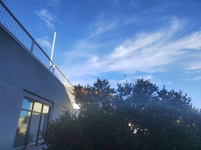
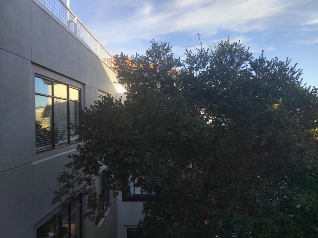
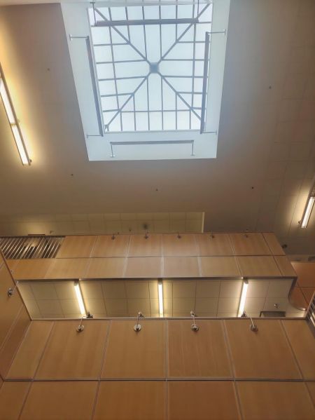
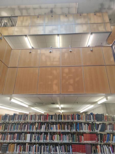
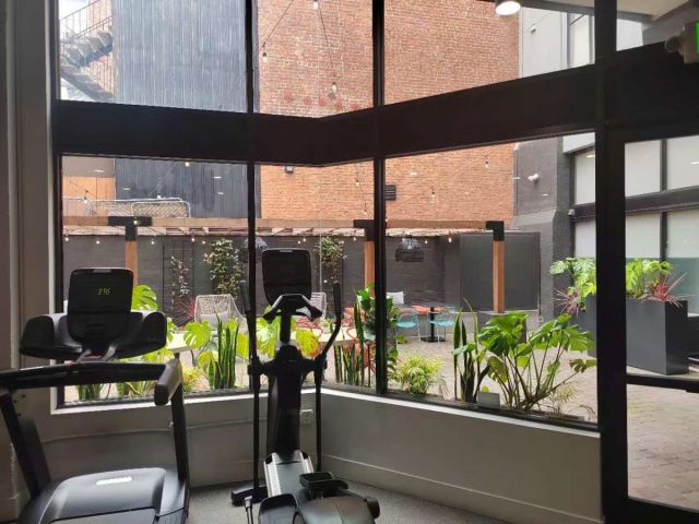
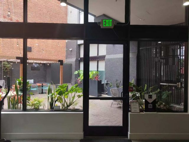
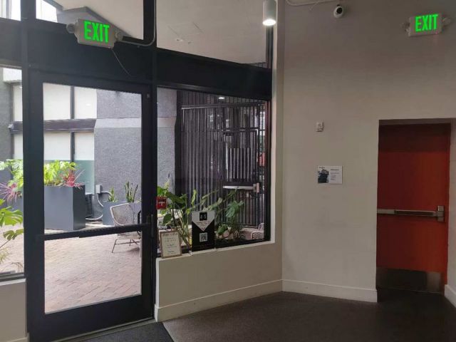
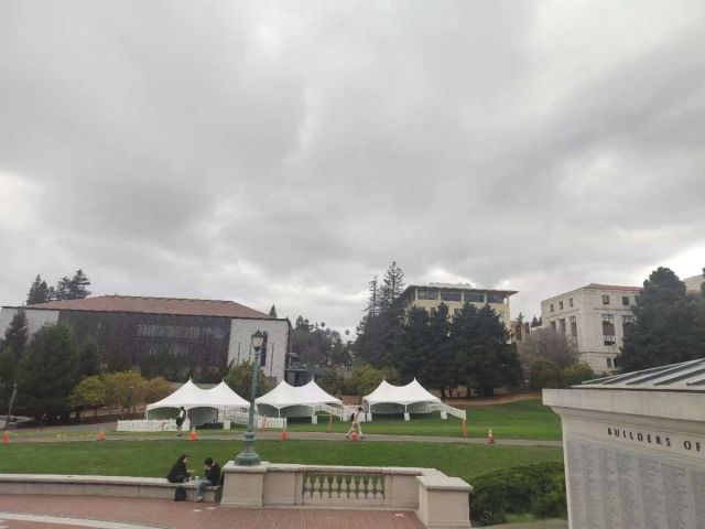
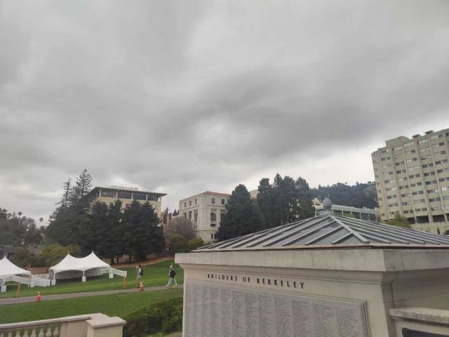
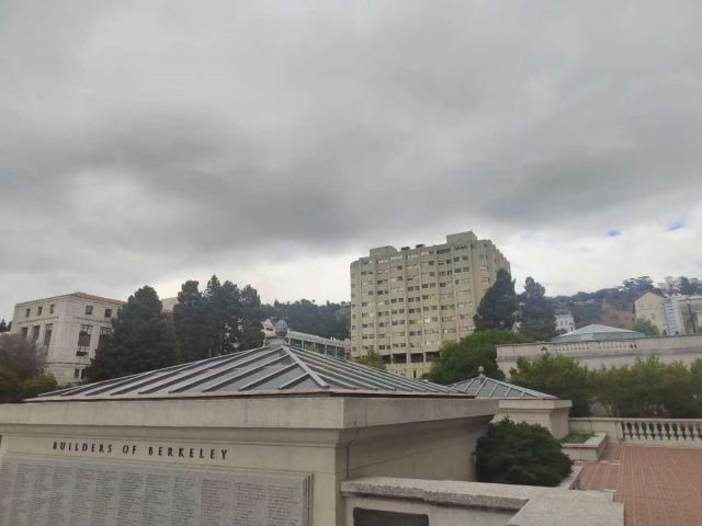
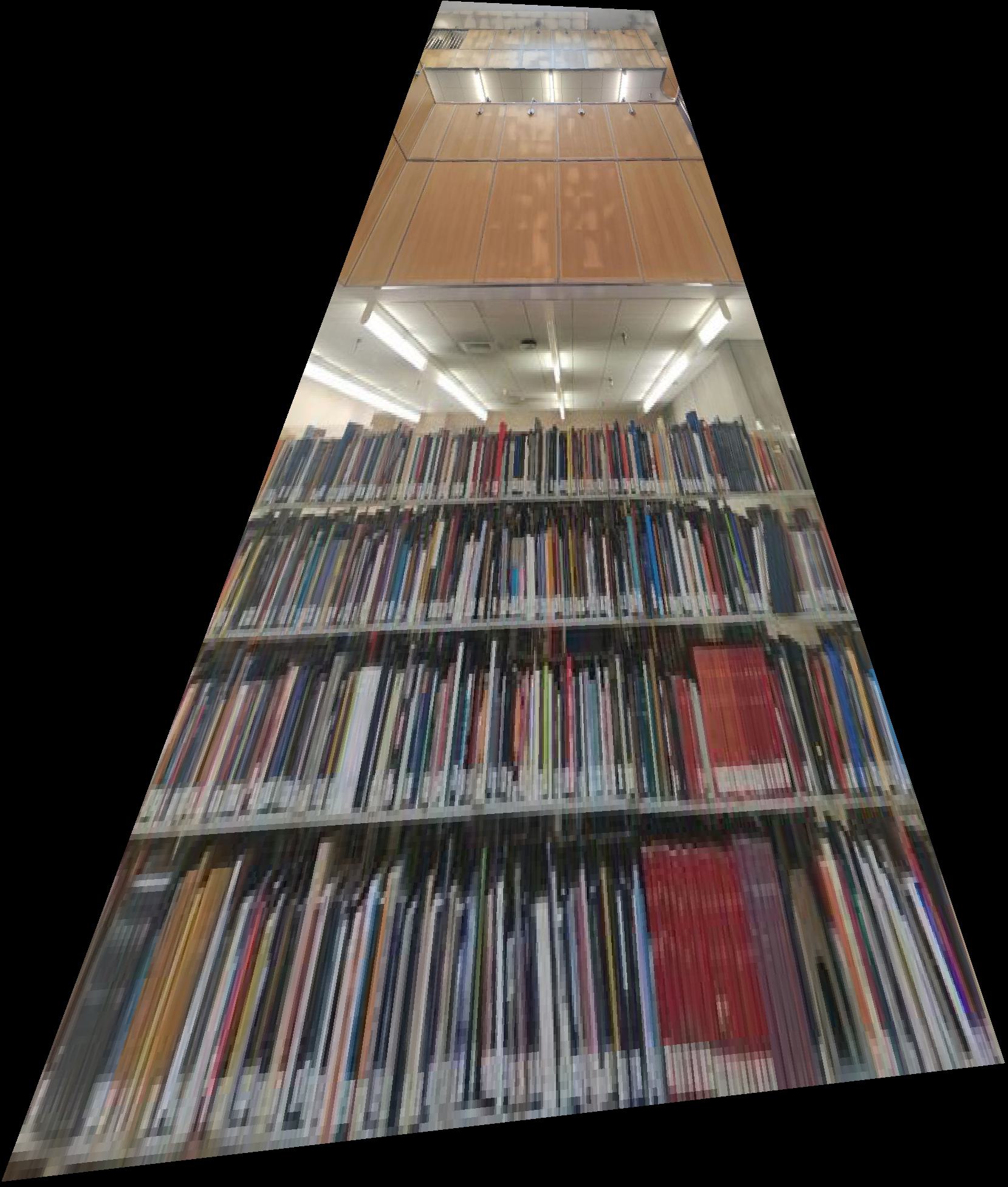
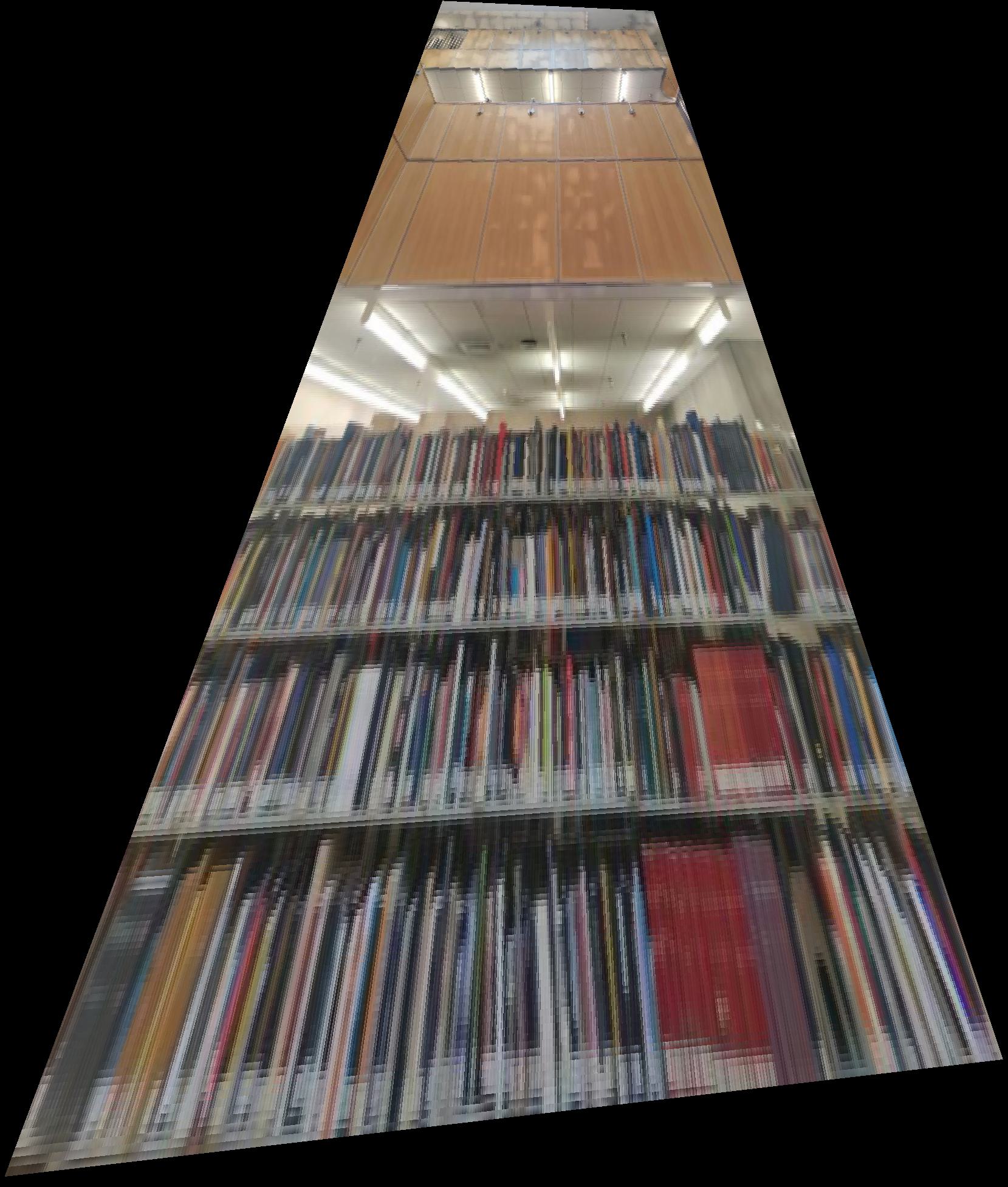
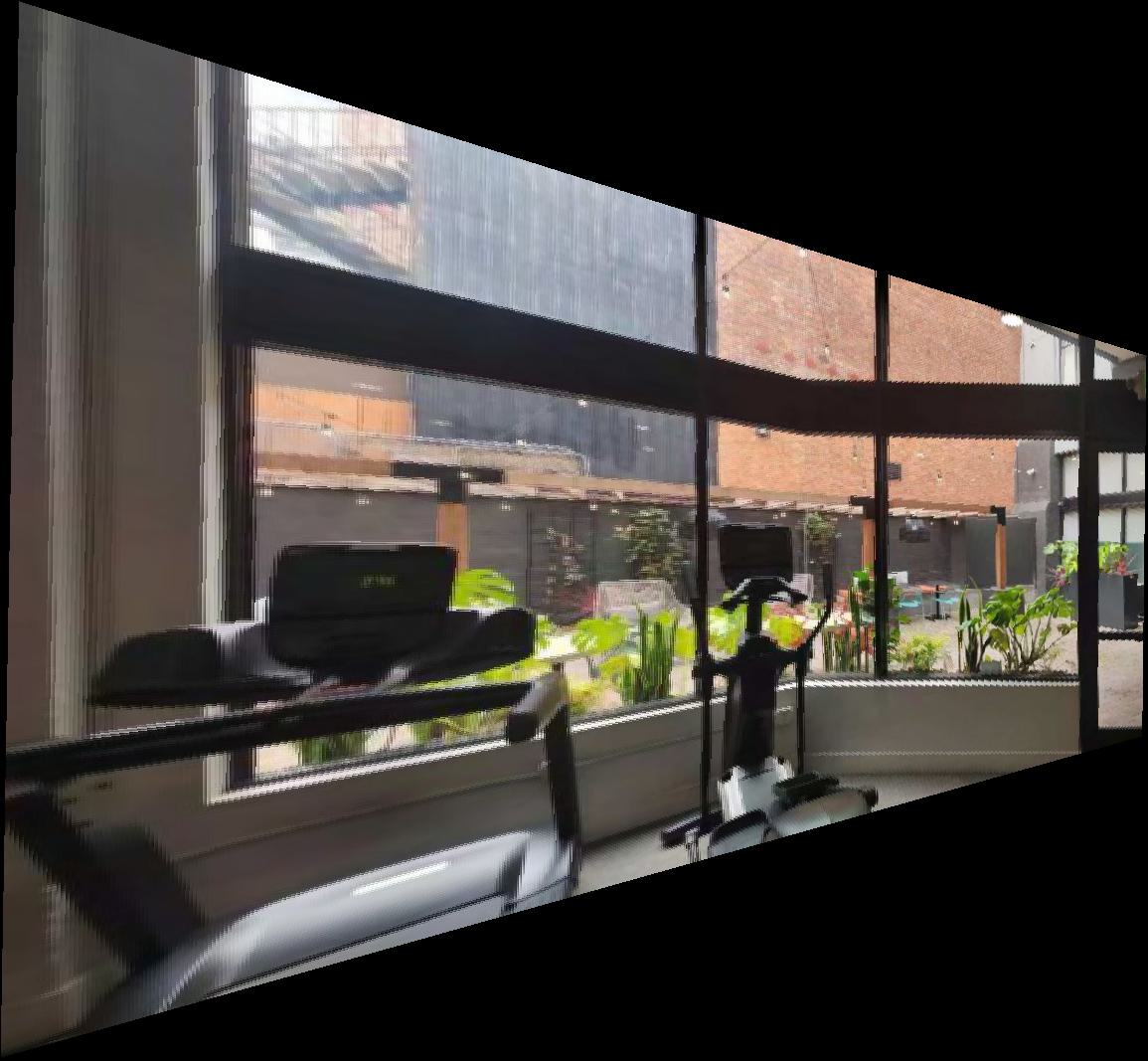
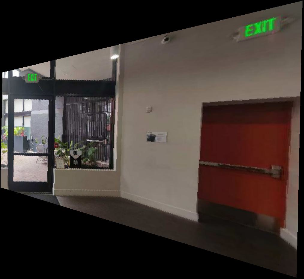
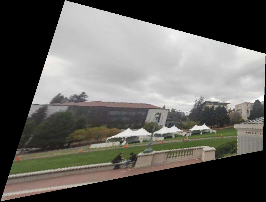
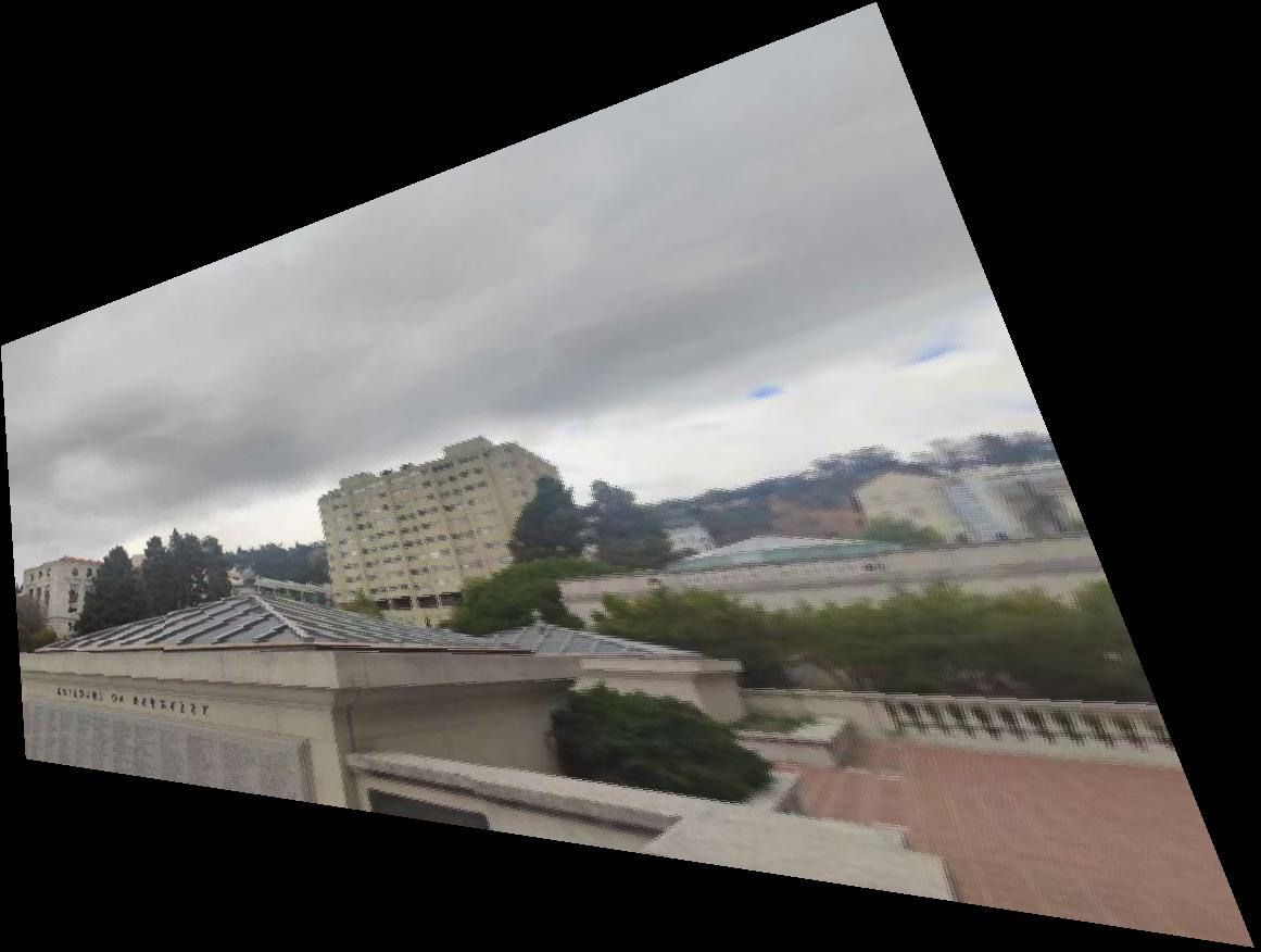
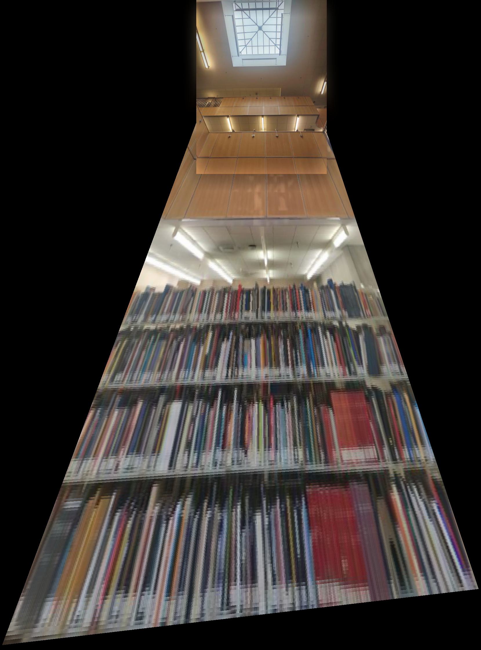
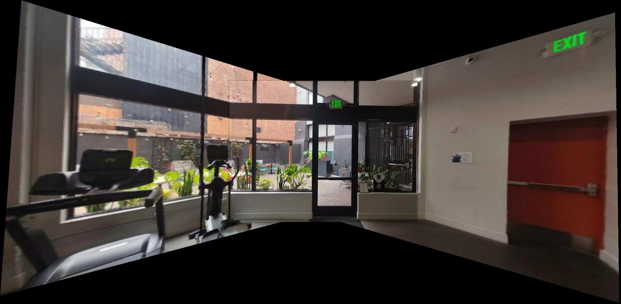
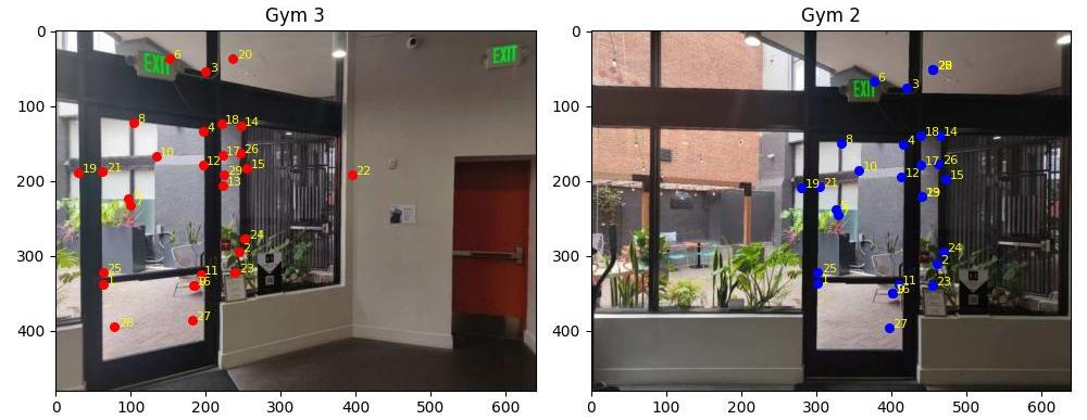
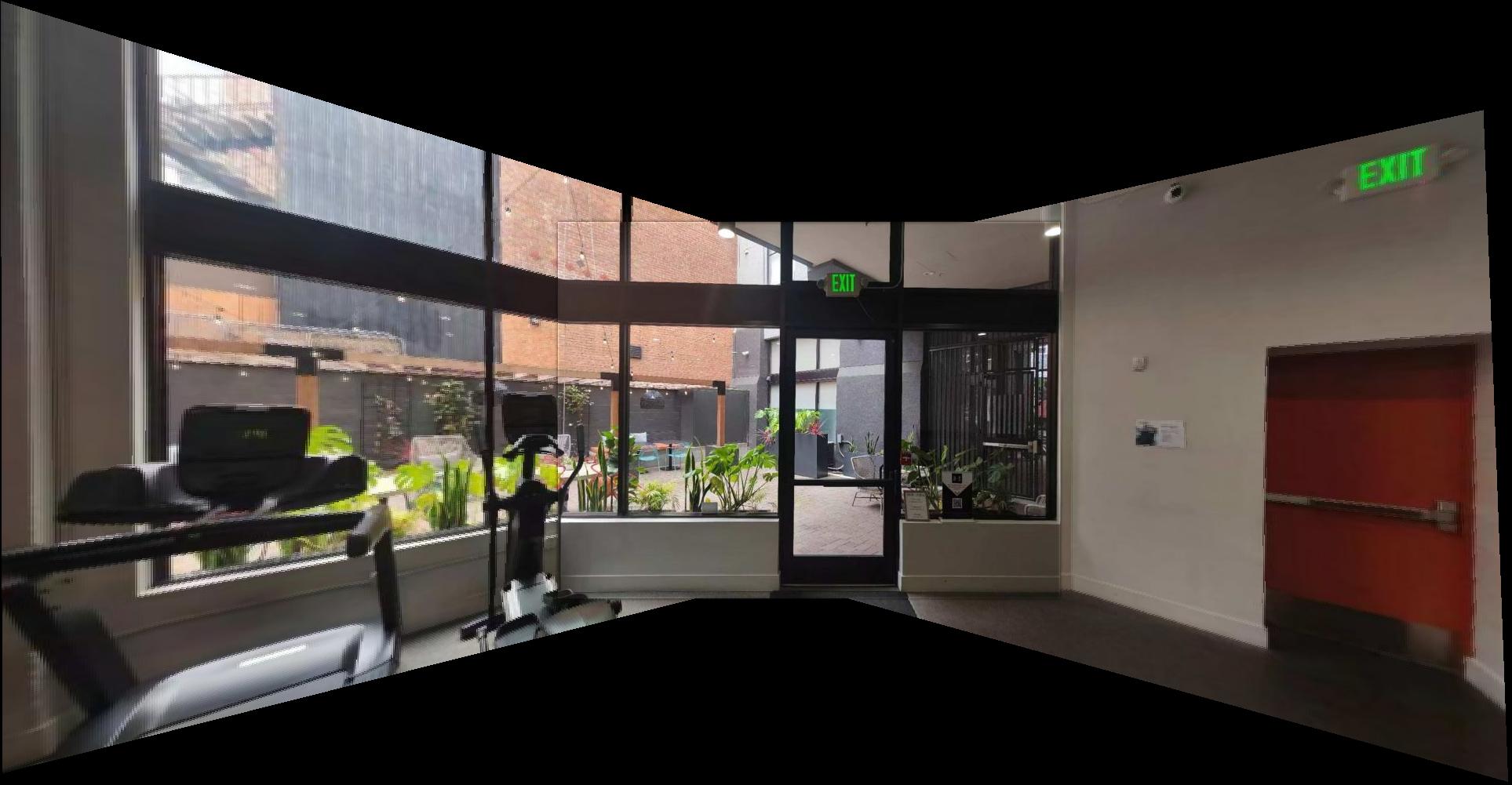
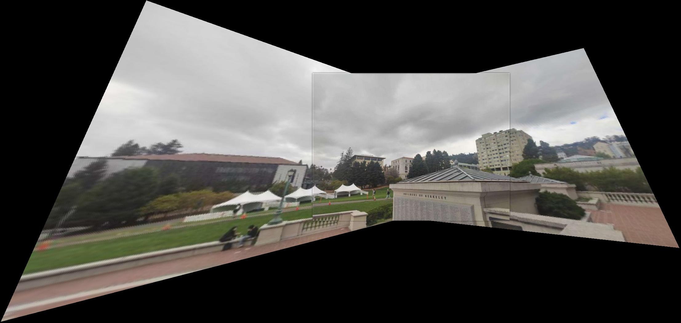
I have acquired three sets of images, with one taken in my apartment's gym, the others taken in the main stack library and in front of the Doe library on campus. The photos from the gym and Doe were taken from a fixed center of projection (COP) with horizontal rotations, while the Main Stack images were taken with vertical rotations around the COP.

A.2: Recover homographies

To recover the homographies, I first manually selected corresponding points on the library images, and computed the homographies between each pair of images. Before implementing the code, some inductions are needed for the final system of equations.

We define the transformation process as \( p^{'} = Hp \): \[ \begin{bmatrix} wu \\ wv \\ w \end{bmatrix} = \begin{bmatrix} a & b & c\\ d & e & f \\ g & h & 1 \end{bmatrix} \begin{bmatrix} x \\ y \\ 1 \end{bmatrix}. \] Then in order to derive the form in \(Au = b\), where \(u = (a \, b \, c \, d \, e \, f \, g \, h)^{T}\), from \[ \begin{cases} wu = ax + by + c\\ wv = dx + ey + f\\ w = gx + hy + 1 \end{cases}, \] by eliminating w, we get: \[ \begin{cases} u = \frac{ax + by + c}{gx + hy + 1}\\ v = \frac{dx + ey + f}{gx + hy + 1} \end{cases}, \] then we can form the system of equations: \[ \begin{cases} u = ax + by + c - gxu - hyu\\ v = dx + ey + f - gxv - hyv \end{cases}, \] so the matrix form for the equations of one corresponding point pair would be: \[ \begin{bmatrix} x & y & 1 & 0 & 0 & 0 & -xu & -yu\\ 0 & 0 & 0 & x & y & 1 & -xv & -yv \end{bmatrix} \begin{bmatrix} a \\ b \\ c \\ d \\ e \\ f \\ g \\ h \end{bmatrix} = \begin{bmatrix} u \\ v \end{bmatrix}. \]

Based on the derived matrix form, we can implement the computeH(im1_pts, im2_pts) function:

  def transformX(p1, p2):
      stack = np.array([[p1[0], p1[1], 1, 0, 0, 0, - p1[0] * p2[0], - p1[1] * p2[0]],
                      [0, 0, 0, p1[0], p1[1], 1, - p1[0] * p2[1], - p1[1] * p2[1]]])
      return stack

  def computeH(im1_pts,im2_pts):
      Xlist = [transformX(p1, p2) for p1, p2 in zip(im1_pts, im2_pts)]
      X = np.vstack(Xlist)
      Y = np.reshape(im2_pts,(-1, 1))
      XTXinv = np.linalg.inv(X.T @ X)
      XTY = X.T @ Y
      h = XTXinv @ XTY 
      H = np.array([[h[0, 0], h[1, 0], h[2, 0]],
                    [h[3, 0], h[4, 0], h[5, 0]],
                    [h[6, 0], h[7, 0], 1]])
      return h, H
  

Now, we can select the corresponding points on the library images, and compute the homographies between each pair of images.

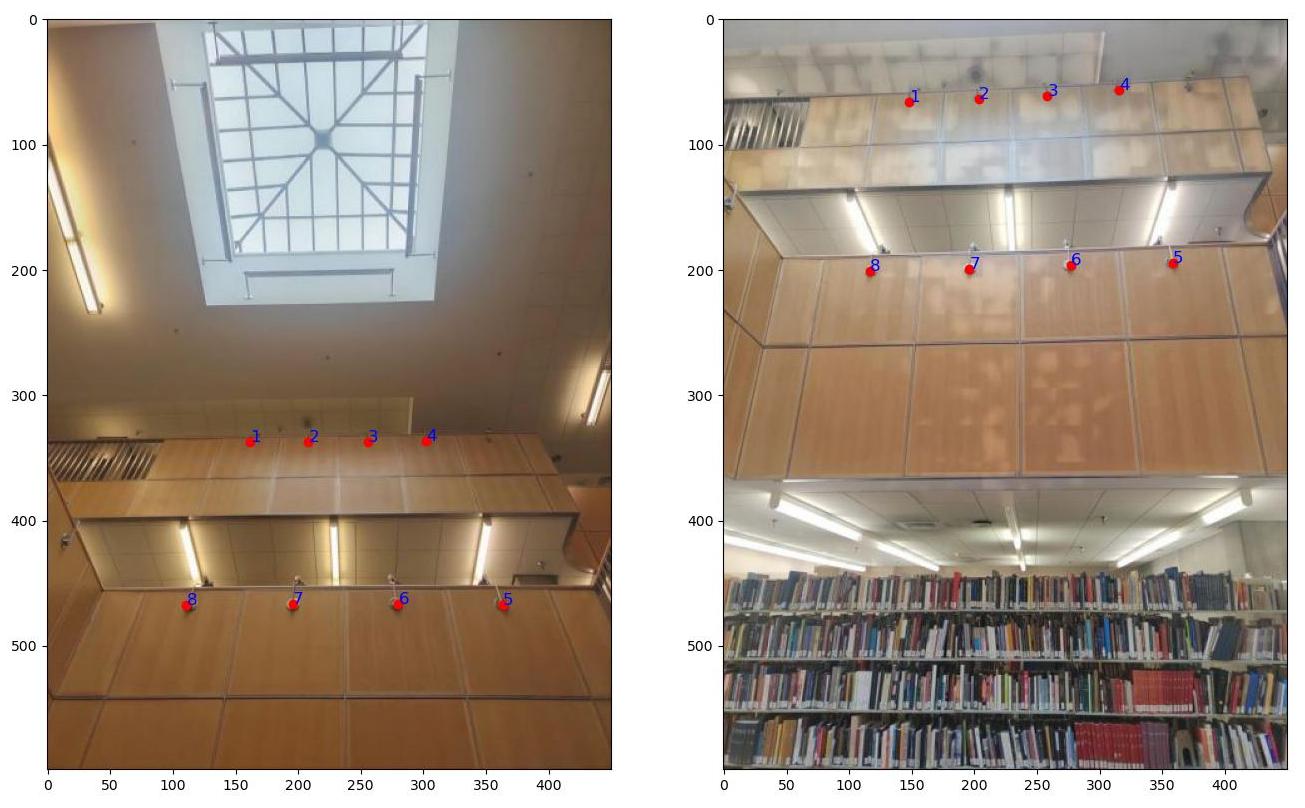
The recovered Homography matrix is: \[ \begin{bmatrix} 8.03065509e-01 & -3.09177799e-01 & 5.05529173e+01\\ 5.84114806e-02 & 2.68021700e-01 & 2.84843095e+02\\ 7.13334305e-05 & -1.33703662e-03 & 1.00000000e+00\\ \end{bmatrix} \]

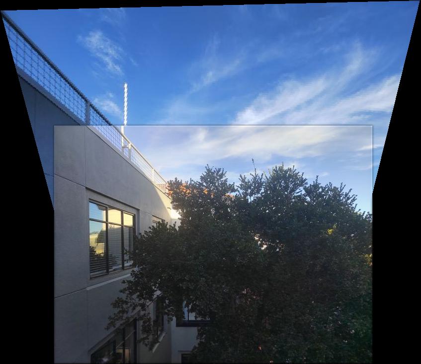
A.3: Warp the images

For image warping, nearest neighbor interpolation and bilinear interpolation are needed after the coordinate transformation, among which the former one round the coordinates on the object image plane after transformation to the nearest pixel value on the original image, while the bilinear interpolation takes the weighted average of the pixel values in the four nearest neighbors.

    def warpImageNearestNeighbor(im, H):
        start = time()
        ## Determine the bounding box of the warped image
        h, w, _ = im.shape
        corners = np.array([
            [0, 0, 1],
            [w, 0, 1],
            [0, h, 1],
            [w, h, 1]
        ]).T
    
        warped_corners = H @ corners
        warped_corners /= warped_corners[2,:]
        xmin, ymin = np.floor(warped_corners[:2].min(axis=1)).astype(int)
        xmax, ymax = np.ceil(warped_corners[:2].max(axis=1)).astype(int)
        h1, w1 = ymax-ymin + 1,xmax-xmin + 1
        im_out = np.zeros((h1 , w1, 3))
        
        ## Transform the coordinates of the warped image to the original image
        x_grid, y_grid = np.meshgrid(np.arange(w1), np.arange(h1)) 
        P_prime = np.stack([x_grid.flatten(), y_grid.flatten(), np.ones(h1 * w1)])
        P_prime[[0],:] +=  np.ones(h1 * w1) * xmin
        P_prime[[1],:] +=  np.ones(h1 * w1) * ymin
        P = (np.linalg.inv(H) @ P_prime).T
        P /= P[:,[2]]

        ## Nearest neighbor interpolation
        for i in range(P.shape[0]):
            if i % 200000 == 0:
                print(f'Processed {i} points')
            x = int(round(P[i,0]))
            y = int(round(P[i,1]))
            if 0 <= x < w and 0 <= y < h:
                im_out[int(i // w1), int(i % w1)] = im[y, x]
        end = time()
        print(f'Finished in {end - start:.2f} s')
        
        ## Return the warped image and the bounding box for stitching
        return im_out, xmin, ymin, xmax, ymax    
  

    def warpImageBilinear(im, H):
        ## Determine the bounding box of the warped image
        
        ## Transform the coordinates of the warped image to the original image

        ## Nearest neighbor interpolation
        for i in range(P.shape[0]):
        if i % 200000 == 0:
            print(f'Processed {i} points')
        x1 = int(np.floor(P[i,0]))
        y1 = int(np.floor(P[i,1]))
        dx = P[i,0] - x1
        dy = P[i,1] - y1
        if 0 <= x1 < w - 1 and 0 <= y1 < h - 1:
            color = im[y1, x1]*dy*dx + im[y1, x1 + 1]*dy*(1 - dx) 
            + im[y1 + 1, x1]*(1 - dy)*dx + im[y1 + 1, x1 + 1]*(1 - dy)*(1 - dx)
            im_out[int(i // w1), int(i % w1)] = color 
        
        end = time()
        print(f'Finished in {end - start:.2f} s')
        
        ## Return the warped image and the bounding box for stitching
        return im_out, xmin, ymin, xmax, ymax    
  

Now we have our warped images. As you can see, the image with nearest neighbor interpolation has more aliasing, while the image with bilinear interpolation is more blurry. In the rest of images, I chose to use bilinear interpolation.

A.4: Blend the images into a mosaic

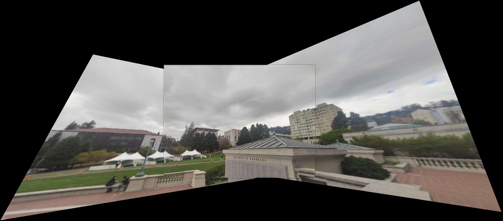
With the warped images as well as their bounding boxes, we can now blend them together to form a mosaic. We first use the bounding boxed to determine the final size of the image mosaic and how the images would fit in the mosaic plane. Furthermore, to soften the image edges, we can use Gaussian kernelw to create a two-layer Laplacain stack for each image as well as the masks covering the area of the images determining the target plane. Here are the final mosaics:

Part B: Feature Matching for Autostitching

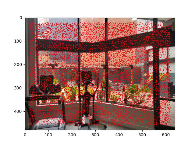
B.1: Harris Corner Detection

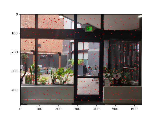
In this section, I used the Harris Corner Detection algorithm to detect corners in images, which is a corner detection operator that works by computing a corner response function for each pixel in the image and thresholding the response function to detect corners. However, the number of local maximums detected by the algorithm are too large, so we need to apply Adaptive Non-Maximal Suppression (ANMS) to choose the corners by the following steps:
 1. Sort the corners by the response function in descending order.
 2. For each corner \(x_i\):
  a. Compute the distance to all other corners.
  b. Find the radius \(r_i = \|x_i - x_j\| \, s.t. f(x_i) < 0.9f(x_j)\).
 3. Find \(N\) corners with the largest radius \(r_i\), here I set \(N = 500\).

The following figure shows the corners detected by the Harris Corner Detection algorithm with or without ANMS:

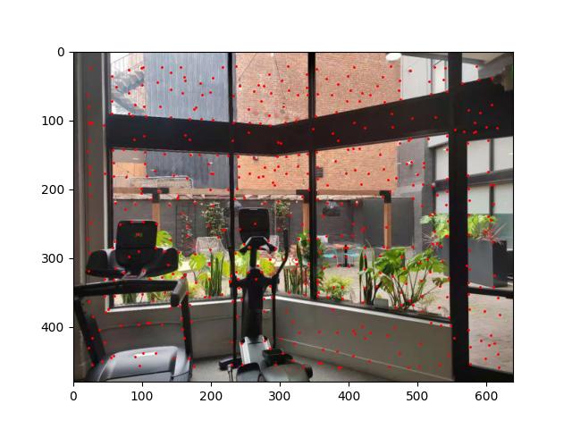
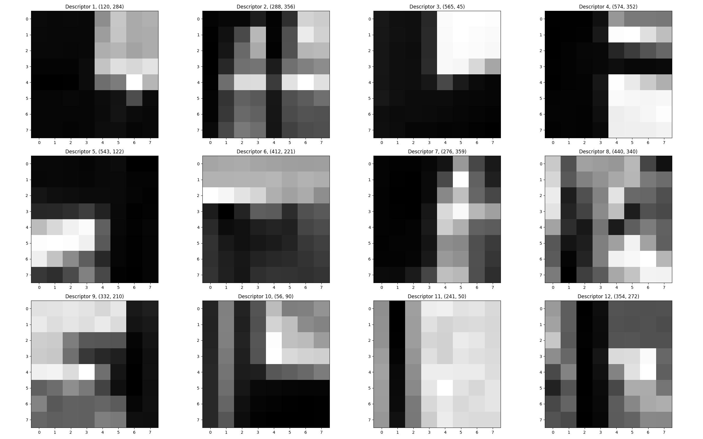
B.2: Feature Extraction

In this section, I used the SIFT algorithm to extract features from images. The descriptor is a 8*8 vector downsampled from the 40 * 40 surrounding area of an interest point that represents the local appearance of the it and is invariant to changes in scale and illumination, here I just implemented the version with vertical and horizontal box edges.

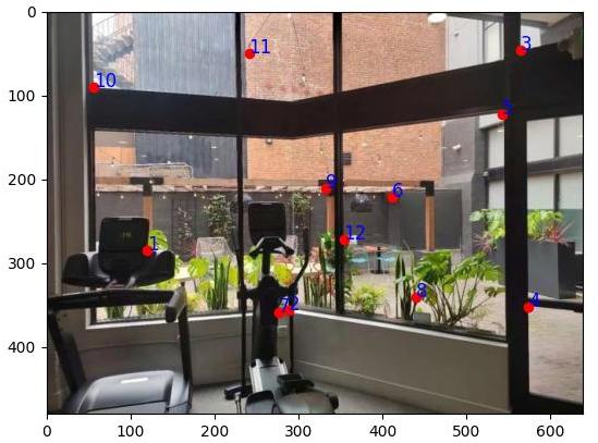
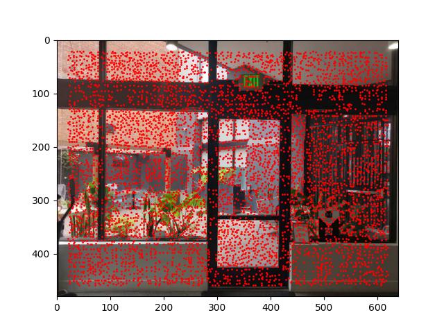
B.3: Feature Matching

To match corresponding features, I used the KNN algorithm to find the top 2 nearest neighbors for each feature point in the two images. The distance metric I used is the Euclidean distance. Then, the feature point pairs with the distance ratio of to the nearest and second nearest neighbors smaller than 0.7 are considered as matched pairs. Since the RANSAC algorithm on the next step is robust as long as the iteration number is suffcient, we can slightly turn up the threshold.

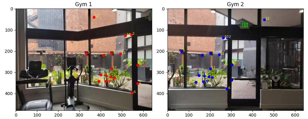
B.4: RANSAC for robust homography

To estimate the homography matrix, I used the RANSAC algorithm. The basic idea is to randomly sample 4 feature point pairs from the matched pairs and estimate the homography matrix using the least squares method. Then, I counted the number of inliers that satisfy the homography transformation. The inlier with the largest number of votes are considered as the final matched pairs. Here, I set the inlier threshold to 2 in Euclidean distance and 4000 as the iteration number.

Apparently, the mosaic with RANSAC is more robust than the manually selected point pairs, since the the edges are less misaligned. However, the phenomenon still exists, probably due to the non-projectional transformation in images shot by real cameras, with distortions on lens edges. Here, due to the lack of edges in the overlapping area of the library images, the feature matching process failed. Therefore, I just replace them with two street photos.