CS180 Project 5

Part A: The Power of Diffusion Models

In this part, the main tasks are some experiments with DeepFloyd IF. Here are some results of image generation:
(seed used: 100)

As you can see, the generated images did not aligned well with the prompt as only part of each prompts are reflected in the images, this is possibly bacause the Inference steps are not enough, or the model itself is not as strong as the latest models such as SORA by OpenAI and Nano Banana by Google.

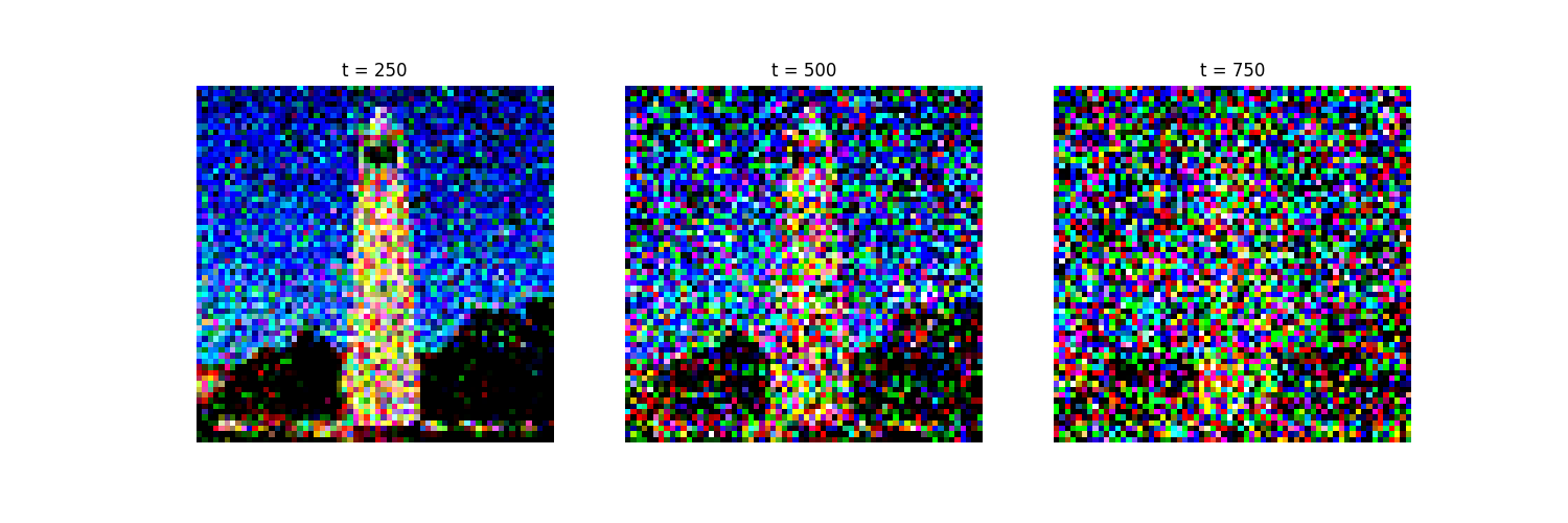
1.1 Implementing the Forward Process

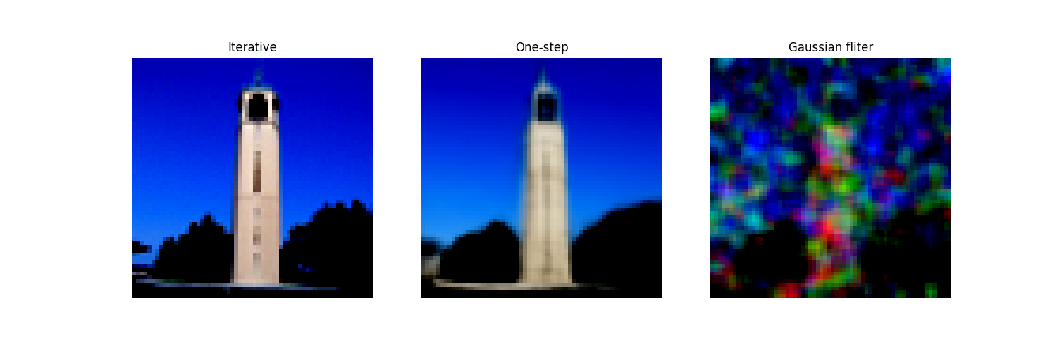
In this part, I implemented the forward process \(x_t = \sqrt{\bar{\alpha_t}}x_0 + \sqrt{1 - \bar{\alpha_t}}\epsilon_t\), here are the results on the Sather Tower image:

1.2 Classical Denoising

Then, traditional Gaussian blurring is applied to the noisy images, and the results are shown below:

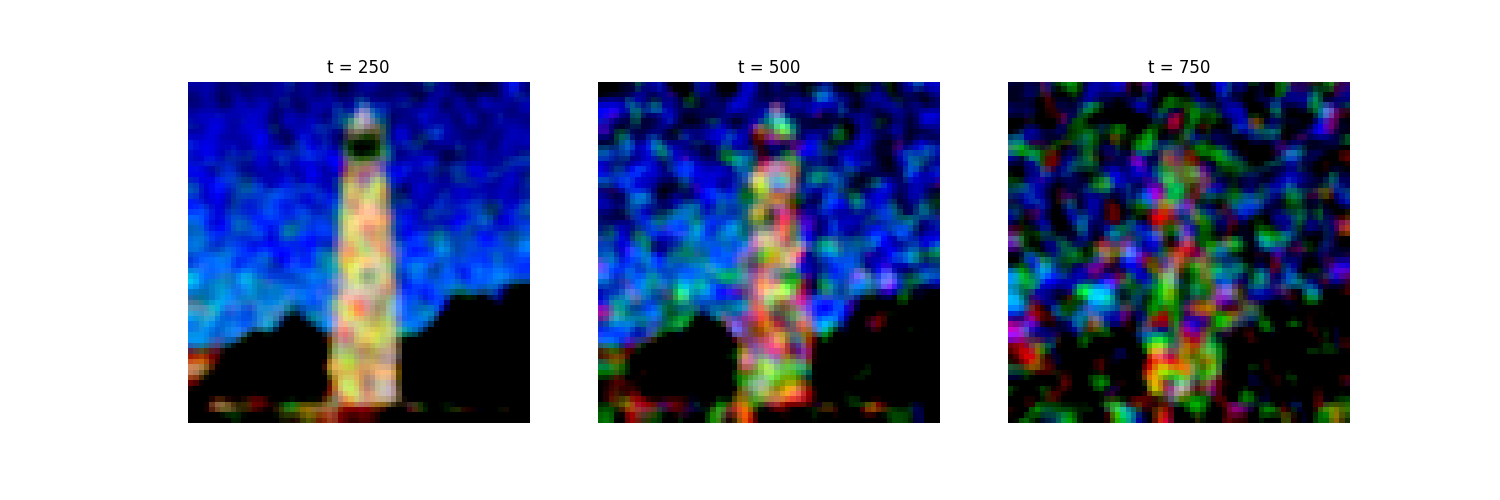
1.3 One-Step Denoising

Apparently, the results of traditional Gaussian blurring is far from satisfaction. Therefore, I implemented the one-step denoising process \(x_{t-1} = \frac{1}{\sqrt{\alpha_t}} \left(x_t - \frac{1 - \alpha_t}{\sqrt{1 - \bar{\alpha_t}}} \epsilon_t\right)\), and the results are shown below:

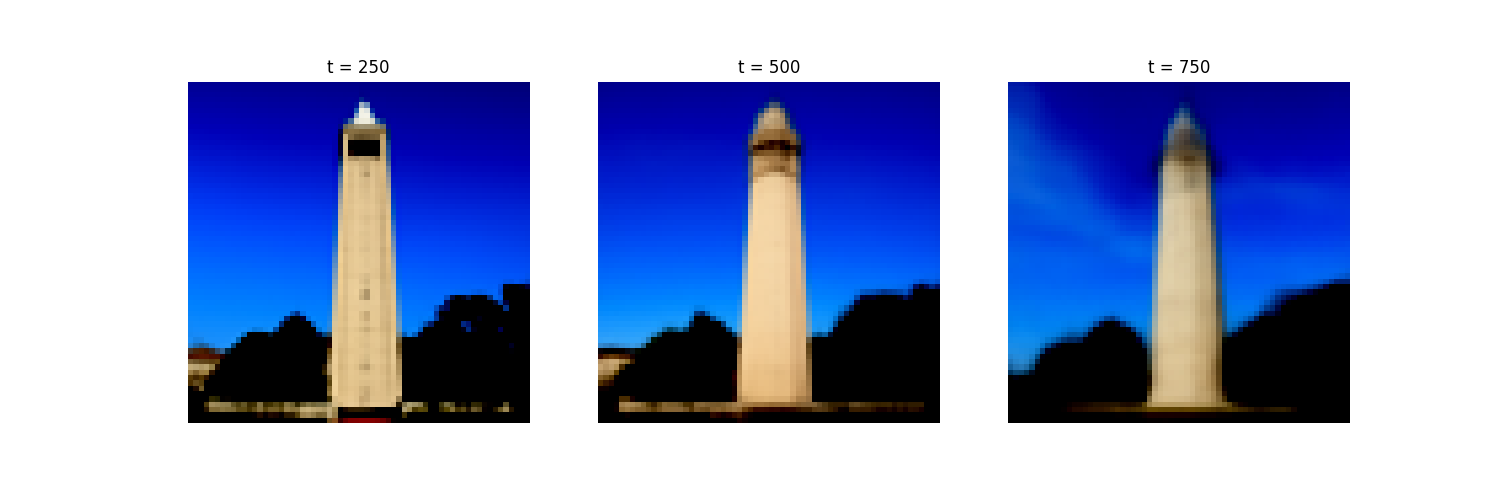
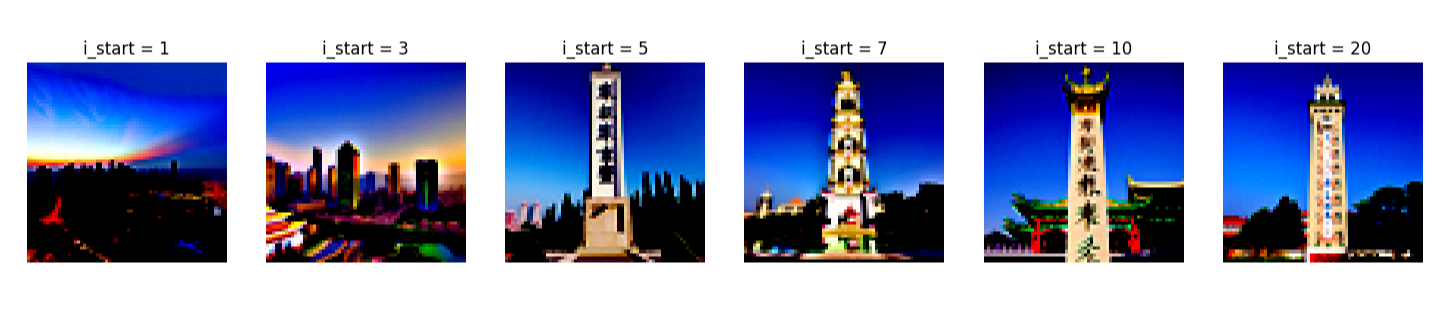
1.4 Iterative Denoising

For higher image quality, I implemented the iterative denoising process \( x_{t'} = \frac{\sqrt{\bar{\alpha}_{t'}\,\beta_t}}{1 - \bar{\alpha}_t} \, x_0 \;+\; \frac{\sqrt{\alpha_t}\,(1 - \bar{\alpha}_{t'})}{1 - \bar{\alpha}_t} \, x_t \;+\; v_\sigma \), and the results are shown below:

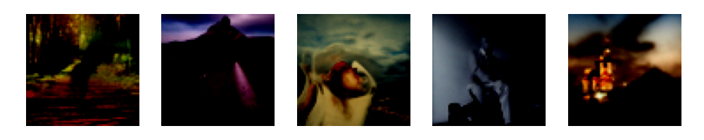
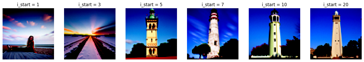
1.5 Diffusion Model Sampling

Start from this section, the experiments are about image generation. By simply sampling, the results are shown below:

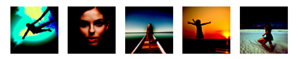
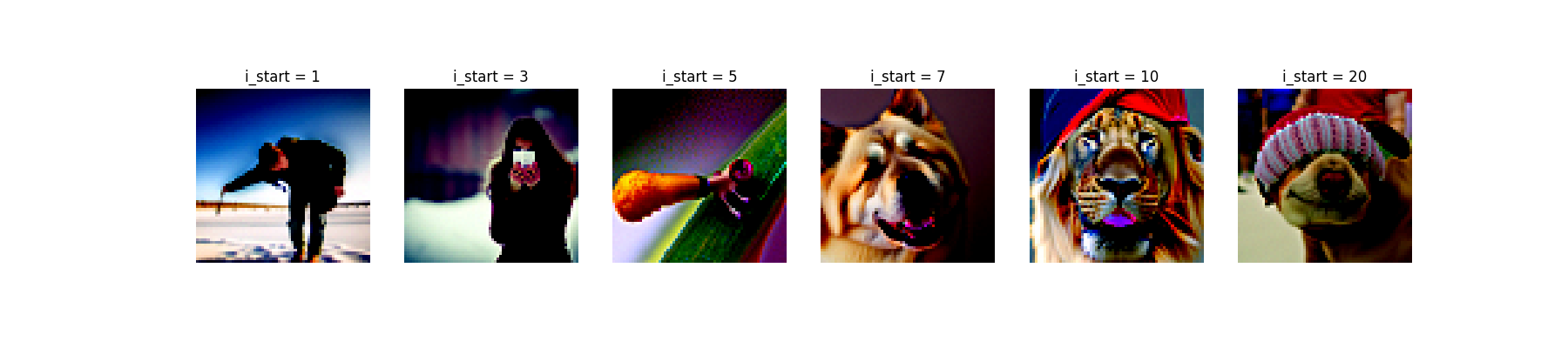
1.6 Classifier-Free Guidance (CFG)

For better image quality, CFG is implemented by adding a conditional term to the denoising process. The results are shown below:

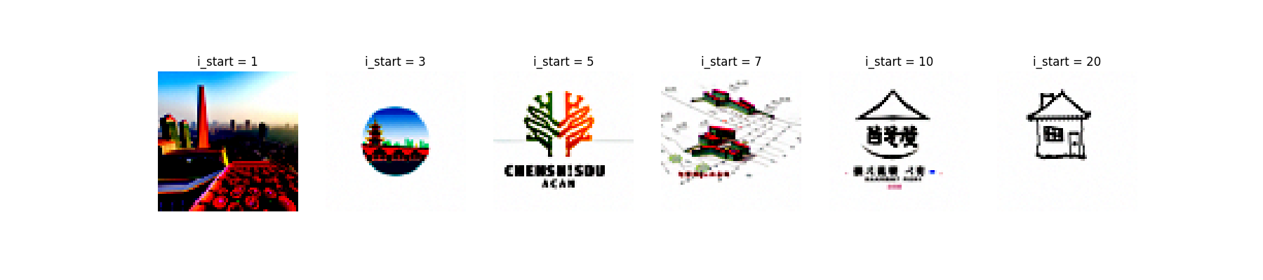
1.7 Image-to-image Translation

1.7.1 Image Editing

With CFG and the default "a high-quality image" prompt, we can edit real or hand-drawn images:

1.7.2 Inpainting

Also, by involving a mask, we can edit the designated area of an image:

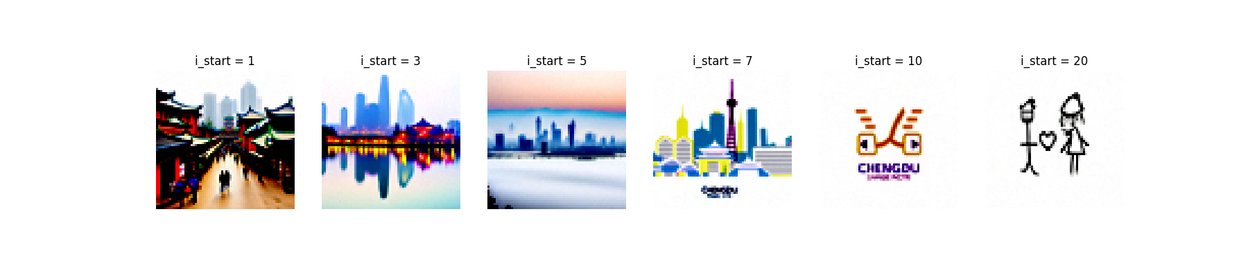
1.7.3 Text-Conditional Image-to-image Translation

By modifying the text prompt, we can generate images a different style. Here I used the prompt "a photo of Chengdu city" for all images.

1.8 Visual Anagrams

To create optical illusions with diffusion models, we will denoise an image \(x_t\) at step \(t\), normally with the prompt \(p_1\), to obtain noise estimate \(\epsilon_1\). But at the same time, we will flip \(x_t\) upside down, and denoise with the prompt \(p_2\), to get noise estimate \(\epsilon_2\). We can flip \(\epsilon_2\) back, and average the two noise estimates. We can then perform a reverse/denoising diffusion step with the averaged noise estimate.

1.9 Hybrid Images

Also, we can take the low frequency component of \(\epsilon_1\) and the high frequency component of \(\epsilon_2\) to create a hybrid image:

Part B: Flow Matching

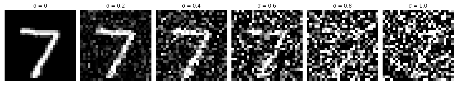
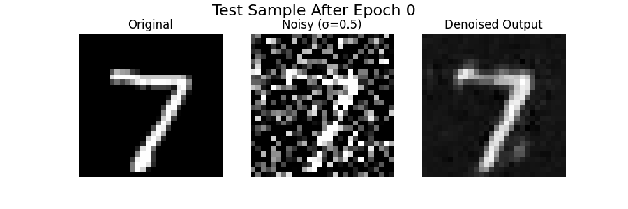
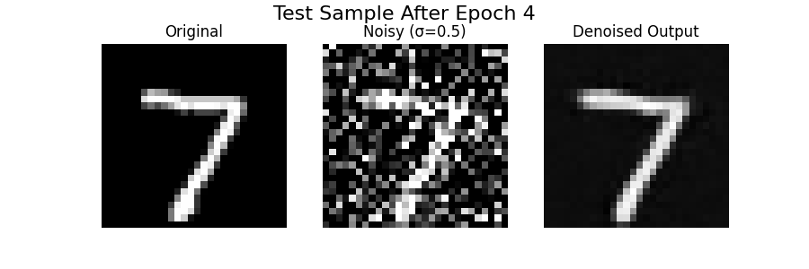
1: Train a denoising U-Net

First of all, the noising process is to add Gaussian noise to the image. Here are some images with different levels of noise added to the same original image:

Then, we train a denoising U-Net to denoise the noisy images. The U-Net is trained with the noisy images as input and the original images as target, and we first set the noise level to 0.5:

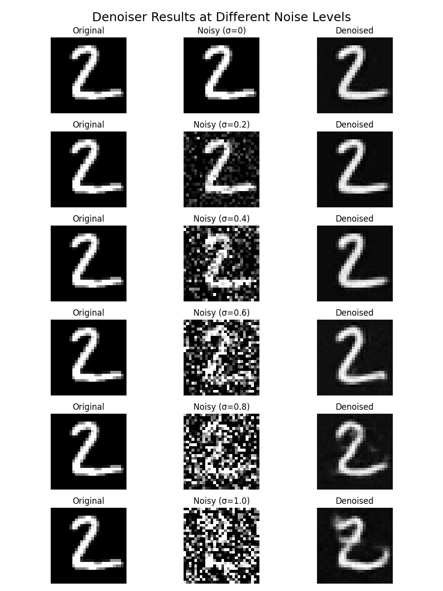
Also, there are sample results on the test set with out-of-distribution noise levels:

Lastly, I tried to denoise pure noisy images. The results are shown below, which is probably an image where all the numbers overlap on each other if the model is fully trained, because the model is trained to recover MNIST digits from pure noise without any input-label correspondence (a one-to-many mapping that cannot be learned), it can only capture the global average structure of the dataset rather than specific digits. As a result, the network collapses toward producing the most common, averaged stroke patterns found across MNIST.

2: Training a Flow Matching Model

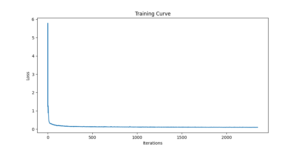
Next, we train a flow matching model to denoise the noisy images and for image generations. To implement that, we need to train a UNet model to predict the `flow' from our noisy data to clean data.

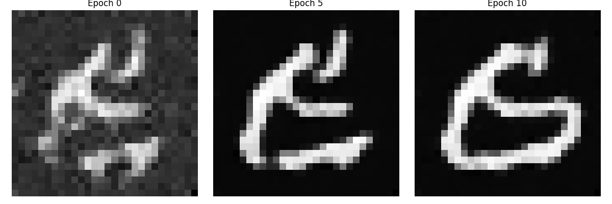
In fact, the sampling result looks quite good. The model can recover the digits from the noisy images. However, we also want to generate an image given a label, so class conditions should be included.

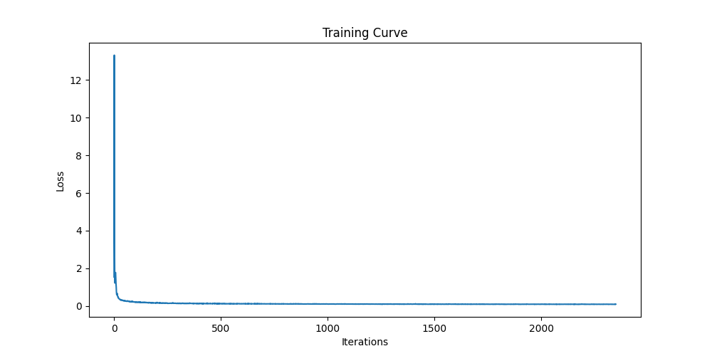
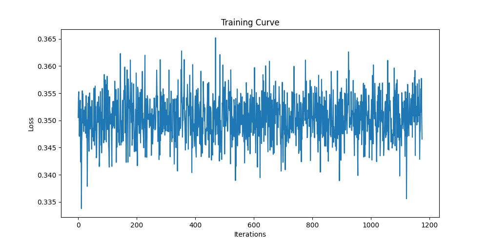
Meanwhile, it was discovered that the learning scheduler with initial learning rate 1e-2 can be replaced by a fixed learning rate 1e-4. Although the convergence is slower, the final results look comparably good to those with a learning scheduler: